
Harmonic Oscillator
Published:
This post is about the basic unit of the Physics, the harmonic oscillator. I start telling you why it is so important in Physics and about the classical version of it. Then, I pass to its quantum version. This “transition” is a good way to see the Correspondence Principle and here I explain why!
This work refers to the initial studies of my Second Scientific Initiation, which project was entitled as Introduction to Particle Physics with Emphasis on Quantum Fluctuations. I have made this work in 2014, under supervision of Professor Attilio Cucchieri, one of the most important people responsible for my first steps in theoretical Physics. At that time (the third year of my undergrad in Physics) I didn’t know nothing about Quantum Mechanics and, that is the first why because, in the first part of that project, I was pretty much interested on it. The second was that, the project aims to study the Casimir effect, which is explained using it (and that you will see in this blog later!).
Why do we need to study the Harmonic Oscillator?
The harmonic oscillator is a key point in Physics (for not to say the most important entity of this science). It is used since basic Physics, to understand simple physical systems (like pendulums, RLC circuits) until the quantization of the free scalar field. Using just a few words, in Classical Physics, the harmonic oscillator model is very important because any mass subject to a force in stable equilibrium acts as a harmonic oscillator for small vibrations.
The Classical Harmonic Oscillator
It consists of a mass $m$ connected with a spring with spring constant $k$. The spring acts with a restoring force $F = - k x$ (Hooke’s law), where $x$ is the displacement of the particle measured from the position at which the spring is “relaxed” [1].
Figure 1 - An example of harmonic oscillator: as it is undamped it undergoes simple harmonic motion.
As this systems has potential energy $V (x) = k x^2/2$, its Hamiltonian $H$ can be written as \begin{equation} H = \frac{p^2}{2 m} + \frac{k x^2}{2} , \end{equation} where $p$ is the particle momentum. This leads to the equation of motion \begin{equation} m \frac{d^2 x}{d t^2} = - k x , \end{equation} which general solution is \begin{equation} x (t) = x_0 \cos (\omega t + \phi) . \end{equation} Here $\omega = \sqrt{k/m}$ is the natural frequency of the oscillator, $x_0$ is the oscillation amplitude and $\phi$ is a phase (given according to the initial conditions of the problem).
The Quantum (1D) Harmonic Oscillator
Analytical solution: Hermite Polynomials
The 1D Quantum Harmonic Oscillator [2, 3, 4] follows the Schrodinger equation \begin{equation} \frac{- \hbar^2}{2m} \frac{d^2 \psi(x)}{d x^2} + \frac{k x^2}{2} \psi(x) = E \psi(x) , \end{equation}
where $\psi(x)$ is the wave function, $\hbar = h/2 \pi$, where $h$ is the famous Planck constant, $E$ is the energy of the particle with mass $m$ and $k$ is the constant of the oscillator. This equation is independent of time and, using the definitions \begin{equation} \xi = \sqrt{\alpha} x, \hspace{0.5cm} \alpha = \frac{m \omega}{\hbar}, \hspace{0.5cm} \gamma = \frac{2E}{\hbar \omega}, \hspace{0.5cm} \omega = \sqrt{\frac{k}{m}}, \label{def} \end{equation} could be rewritten as \begin{equation} \left (\xi^2 - \frac{d^2}{d \xi^2} \right) \psi(\xi) = \gamma \psi(\xi). \label{eq:equacaodeautovalores} \end{equation}
In order to solve it you can use the famous ladder operators: the lowering operator $A$ and the raising operator $A^{\dagger}$. In particular, we can write the eigenvalue equation \begin{equation} \widetilde{H} \psi_{\gamma}(\xi) = \gamma \psi_{\gamma} (\xi), \label{valor} \end{equation} where \begin{equation} \widetilde{H} = \frac{2}{\hbar \omega} H = \xi^2 - \frac{d^2}{d\xi^2} = \frac{A A^{\dagger} + A^{\dagger} A}{2} = A^{\dagger} A + 1 \end{equation} \begin{equation} A = \xi + \frac{d}{d\xi} , \end{equation} \begin{equation} A^{\dagger} = \xi - \frac{d}{d\xi}. \end{equation} The most known relation concerning to these operators is \begin{equation} \left[A, A^{\dagger}\right] \equiv AA^{\dagger} - A^{\dagger}A = 2 \end{equation} and the reason behind their names is because, for example, they raise and low the quantum states: $\gamma \in [0, \infty)$.
The eigenvalue equation that corresponds to the minimum of energy, or, in other words, the “lowest rung” is \begin{align} A \psi_0 (\xi) = \left(\xi + \frac{d}{d\xi}\right)\psi_0(\xi) = 0 , \end{align} with solution given by \begin{equation} \psi_0(\xi) = C e^{-{\xi^2/2}} \end{equation} and energy \begin{equation} E_0 = \frac{\hbar \omega}{2}. \end{equation}
In this way, applying $n$ times the operator $A^{\dagger}$ in $\psi_0(\xi)$ gives all other states, that is \begin{equation} \psi_n (\xi) = C_n (A^{\dagger})^n e^{-{\frac{\xi^2}{2}}} , \end{equation} \begin{equation} E_n = \left( n + \frac{1}{2} \right) \hbar \omega . \end{equation} Analytically, we can see the Hermite polynomials of degree $n$ and write \begin{equation} \psi_n(x) = C_n e^{-\frac{\alpha x^2}{2}} H_n(\sqrt{\alpha} x), \end{equation} \begin{equation} C_n = \sqrt{\frac{\sqrt{\alpha}}{2^n n! \sqrt{\pi}}}. \end{equation} which completes the solution for the 1D Quantum Harmonic Oscillator.
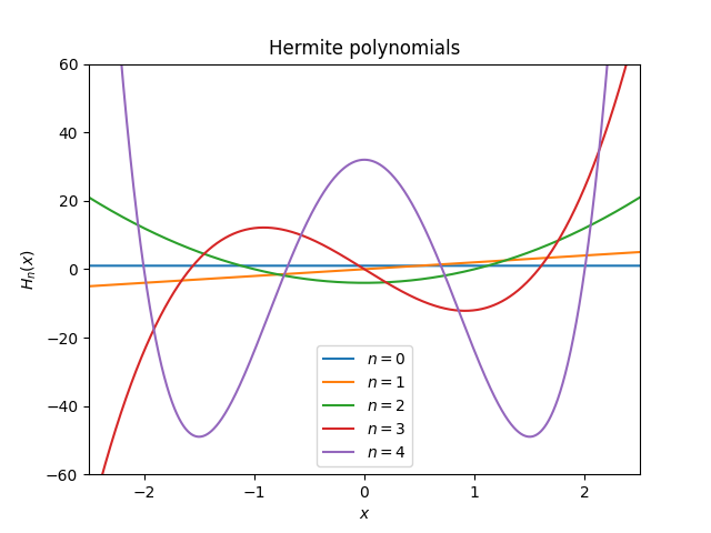
Figure 2 - A visual representation of the Hermite polynomials.
In Quantum Mechanics we do not measure the wave functions (which could be thought as a mathematical artifact to represent the physical systems), but, instead of this, we measure the Probability Density $|\psi (x, t)|^2$, due to Max Born (1926). Thus, the probability of finding a particle in some region $a \le x \le b$ in the time $t$ is \begin{equation} P[a,b] = \int_{-a}^{b} \left| \psi(x,t) \right|^2\, dx. \end{equation} This entity synthesizes the probabilistic interpretation of the wave function.
In the case of the 1D Harmonic oscillator, the wave function does not depends of time, but we have the probability density $|\psi_n (x)|^2$ of finding the particle in space, for each energy level.
Figure 3 - Wave functions $\psi_n (x)$ (on the left) and probability density function $|\psi_n (x)|^2$ (on the right) for the energy levels $n = [0, 3]$ of 1D Quantum Harmonic Oscillator. In the center of the figure, you can see the eigenvalues $E_n$ for the energy inside the potential energy.
Numerical Solution: Numerov Method
Of course the above solution is pretty nice, but, it is in some sense “possible” due to Hermite polynomials. However, what happens when we don’t have access to analytical functions? One possible way to circumvent this problem is to use Numerical methods. Numerical methods are mathematical tools used to solve problems numerically. Ok, duh, but, what does it means? I really like to think about this as we are solving, for instance, some differential equation, by steps, dividing the problem in some little pieces (like Jack, the ripper) that, when put together in a smart way, represents exactly the solution to the problem.
In the case of the quantum harmonic oscillator we can use the Numerov’s Method. But why does this have this name? The method was developed by the Russian astronomer Boris Vasil’evich Numerov. Numerov’s method is (of course) a numerical method to solve ordinary differential equations of second order in which the first-order term does not appear. More specifically, equations like \begin{equation} \frac{d^2 y}{dx^2} = y’’ = -g(x)y(x) + s(x), \end{equation} where $g(x)$ and $s(x)$ are known functions which are independent from initial conditions \begin{equation} y(x_0) = y_0 , \hspace{1cm} y’(x_0) = y_0’. \end{equation}
And, for our lucky, that is exactly the type of the differential equation from the Quantum Harmonic Oscillator!
As I said, we can solve the problem in question by parts and, in this way, the differential equation could be discretized considering $N$ points $x_1, x_2, \dots, x_N$ equidistant in some given interval $[a, b]$. The discretization could be proved using Taylor expansion to write $y_i = y (x_i)$ in terms of $y_{i - 1}$, $y_{i - 2}$ and the known functions $g_i = g (x_i)$ and $s_i = s (x_i)$. This allows the iteractivelly computation of $y_i$ (for all values of $i$) using $y_0$ and $y_1$ fixed or, equivalently, using the initial conditions $y (x_0)$ and $y’ (x_0)$. The so expected expansion is given as follows \begin{equation} y_{i-1} = y_i - y_i’ \Delta x + \frac{1}{2}y_i’’ {\Delta x}^2 - \frac{1}{6}y_i’’’ {\Delta x}^3 + \frac{1}{24}y_i’’’’ {\Delta x}^4 - \frac{1}{120} y_i ‘’’’ {\Delta x}^5 + O[{\Delta x}^6] \end{equation} \begin{equation} y_{i+1} = y_i + y_i’\Delta x + \frac{1}{2}y_i’’ {\Delta x}^2 + \frac{1}{6}y_i’’’ {\Delta x}^3 + \frac{1}{24}y_i’’’’ {\Delta x}^4 + \frac{1}{120} y_i’’’’ {\Delta x}^5 + O[{\Delta x}^6], \end{equation} where $y_{i-1}$ and $y_{i+1}$ represent, respectively, the anterior and posterior points with respect to $y_i$. After some algebra, we can find the Numerov’s expression as
\begin{equation} y_{i+1}\left[ 1 + g_{i+1}\frac{(\Delta x)^2}{12}\right] = 2y_i \left[ 1 - 5g_i \frac{(\Delta x)^2}{12}\right] - y_{i-1} \left[ 1 + g_{i-1} \frac{(\Delta x)^2}{12} \right] + \end{equation}
\begin{equation}
- (s_{i+1} + 10s_i + s_{i-1}) \frac{(\Delta x)^2}{12} + O[(\Delta x)^6]. \end{equation} This gives each value of $y_{i + 1}$ using the previous two numbers.
The reason why we can use this method to solve the Schrodinger equation is because we can identify \begin{equation} g(x) = \frac{2m}{\hbar^2} [E - V(x)], \hspace{1cm} s(x) = 0. \end{equation} using the definitions \begin{equation} g_i \equiv \frac{2m}{\hbar^2} [E - V(x_i)], \hspace{1cm} f_i \equiv 1 + g_i \frac{(\Delta x)^2}{12} . \end{equation}
Then, the Numerov expression is given by \begin{equation} y_{i+1} = \frac{(12 - 10f_i)y_i - f_{i-1}y_{i-1}}{f_{i+1}}. \end{equation}
For the Quantum Harmonic Oscillator $V (x) = k x^2 / 2$ and the initial points $y_0 = y(x_0) = y(0)$ and $y_1 = y(x_1)$ are find, for each eigenfunction, using the parity symmetry of the wave equation $\psi_n (x)$, i.e., $\psi_n (x)$ = $(-1)^n$ $\psi_n (-x)$. Therefore we choose \begin{equation} odd \hspace{0.2cm} n \Longrightarrow y_0 = 0, \hspace{2.6cm} y_1 = arbitrary \end{equation} \begin{equation} even \hspace{0.2cm} n \Longrightarrow y_0 = \hspace{0.1cm}arbitrary, \hspace{1.1cm}y_1 = \frac{(12 - 10f_0)y_0}{2f_1}. \end{equation} It is interesting to notice that, using the symmetry of the parity of the eigenfunction, we can only compute the analytical solution in the interval $x \in [0, x_{max}]$, where $x_{max}$ is the maximum value of $x$. The complete eigenfunction if obtained imposing the symmetry of the parity (positive or negative) for the numerical solution. In my solution, for all values of $n$ the point $x_{max}$ was fixed using $n = 30$.
Here comes an importamt step in this solution, that is the way that we used to obtain the eigenvalues of the energy $E_n$. We have considered values in the interval $[0, 30.5]$ (as we stop in $n = 30$) which are splited in interval of $d E = 10^{- 2}$. We were looking for well behaved wavefunctions (functions which does not “explode” for higher values of $x$). This task was done analyzing the behavior of the derivative of the function in $x_{max}$ observing that, when we pass behind an eigenvalue of energy, the value of its derivative inverted it signs.
| n | Theoretical Energy | Obtained value |
|---|---|---|
| 0 | 0.5 | 0.50 |
| 1 | 1.5 | 1.50 |
| 2 | 2.5 | 2.50 |
| $\vdots$ | $\vdots$ | $\vdots$ |
| 30 | 30.5 | 30.50 |
Analytical and Numerical comparison
After computing the eigenenergies, we computed the respective eigenfunctions and compared with the analytical results. This was made for different $n$s and $|\psi_n(x)|^2$s. See that the errors are around just $10 \%$ (for $n = 30$), in the residue plots.
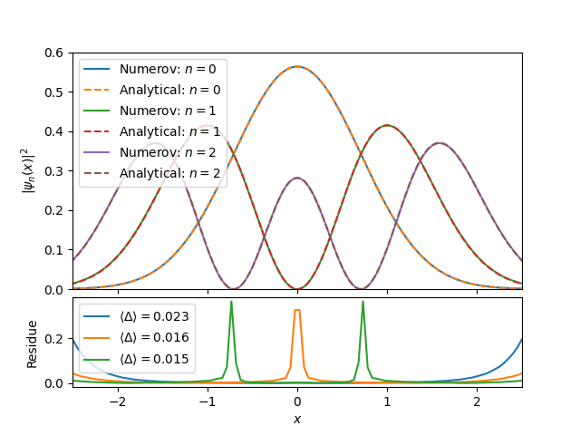
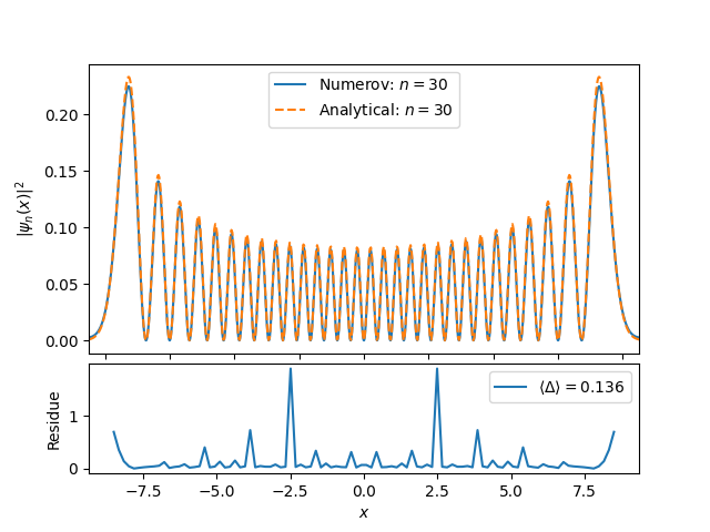
Figure 4 - Comparison between analytical (solution using the Hermite polynomials) and numerical (obtained using Numerov’s method) for $n = [0, 1, 2, 30]$.
The Correspondence Principle
The main difference between the classical and quantum analysis is in the way that they describe the particle dynamics. In the first case, we consider the position and velocity of some particle according to time. In the second, we describe the probability of finding some particle in some position and time. Apparently, those analysis have nothing in common, but, we can compare both thinking about the probability density. Classically, the probability density could be seen as the inverse of the velocity of the particle, which is higher in the extremes of the oscillation (as you will see for the harmonic oscillator). At the same time, it is exactly what we measure in Quantum Mechanics.
At this point the Correspondence Principle enters, saying that any physical phenomenon described in Quantum Mechanics reproduce a Classical partner in the limit of higher quantum numbers. This is equivalent to say that, for higher energies, the quantum probability is compared to classical probability [5, 6].
The case of the 1D Harmonic Oscillator
Figure 5 - Some simple comparison of the probability density functions for the 1D Harmonic Oscillator Classical and Quantum for the energy levels $n = [0, 1, 2, 3, 10]$.
In the case of the 1D Harmonic Oscillator we can compare the classical and quantum solution for any quantum number $n$, simply using any wave function for the respective $n$. But, how we can see the classical probability density?
If we take the classical and quantum energy as the same \begin{equation} \frac{k{x_0}^2}{2} = \frac{\omega^2 m {x_0}^2}{2} = \left( \frac{1}{2} + n \right) \hbar \omega, \end{equation} we obtain \begin{equation} \left| x_0^{(n)} \right| \leq \frac{\hbar \sqrt{2n + 1} }{m \omega} = \frac{\sqrt{2n + 1}}{\alpha}, \label{mod} \end{equation} where $\alpha = m\omega/\hbar$. It is interesting to see that, the amplitude $x_0^{(n)}$ vary according to the level of energy $n$ of the particle, that means that, when we increase the energy level, we increase the total energy of the system. Therefore, we can define the classical probability density $\rho_n (x)$ of finding the particle inside the interval $[x, x + dx]$ as \begin{equation} \rho_n(x) dx = \frac{dx}{|v(t)|} = \frac{dx}{x_0^{(n)} \omega |sen(\omega t)|} , \end{equation} which is the inverse of its velocity $v (x)$.
My comparison is given bellow. It shows an amazing correspondence, as we expected.
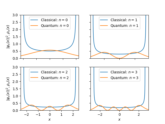
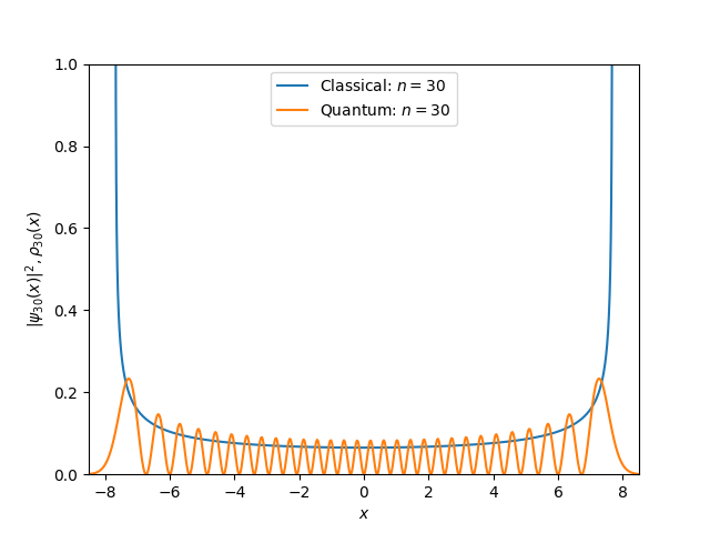
Figure 6 - My comparison to prove the Correspondence Principle. Here you can see the classical probability to find the particle and the quantum probability density function for $n = [0, 1, 2, 3, 30]$.
Code
The codes for this work (including the numerical and analytical solutions) are presented in my repo: https://github.com/natalidesanti/harmonic_oscillator.
References
[1] Classical Mechanics, Taylor, J. R. 2005.
[2] R. Resnick, Introdução a Relatividade Especial, Poligono (São Paulo), 1971.
[3] S. Gasiorowicz, Quantum Physics, John Wiley (New York), 1996.
[4] C. Tannoudji, Quantum mechanics, John Wiley (New York), 1977.
[5] The Correspondence Principle and the Quantum Oscillator. Available in the page.
[6] P. Giannozzi, Numerical Methods in Quantum Mechanics, Available in the page, 2014.