Schwarzschild Black Holes

This post is dedicated to the Schwarzschild solution of Einstein’s equations. Here I will follow a simple way to deduce it and show why this solution arises to what we call as the basic kind of black hole: the Schwarzschild Black Holes.

This post is related with the first steps of my Masters’ degree, in Black Hole Thermodynamics, that I have worked from 2016 to 2018, under supervision of Professor Raphael Santarelli.

The Einstein’s Equations

The core from General Relativity is attributed to Einstein, due to his field equations, from 1915. Those equations related the curvature of the spacetime, represented by the Einstein tensor $G_{\mu \nu}$, with the matter and energy, given by the stress tensor $T^{\mu \nu}$ [1]. The Einstein tensor equation can be written as \begin{equation} G_{\mu \nu} \equiv R_{\mu \nu} - \frac{1}{2} R g_{\mu \nu} = - \frac{8 \pi G}{c^4} T_{\mu \nu} , \end{equation} where $R_{\mu \nu}$ is the Ricci tensor, $R$ is its trace, $g_{\mu \nu}$ is the metric tensor, $G$ is the gravitational constant and $c$ is the speed of light. It is usual to define $G = c = 1$ and recover the Physical units at the end of the computations, and I will do this here as well.

The general idea is that, those equations are extremelly non-linear, which makes those solutions hard to find. However, once we use symmetry, the solutions are more straightforward to find. And this was made by Schwarzschild, in 1916. This solution consists in a spacetime to represent a spherical symmetry, static and asymptotically flat for a gravitational empty field around a spherical massive object [2].

Pursuing the solution

First we need to choose some coordinates to work with. Because we want to work with spherical symmetry, let’s use the spherical coordinates and time as \begin{equation} (t, r, \theta, \phi) . \end{equation} Using the tensor notation, we can postulate the line element as \begin{equation} ds^2 \equiv g_{\mu \nu} dx^{\mu} dx^{\nu} = A(r) dt^2 - B(r) dr^2 - r^2 [d\theta^2 + \sin^2 \theta d\phi^2] , \end{equation} where I have used Einstein summation convention (a notational convention that implies summation over the indexed terms in the formula) and the functions $A (r)$ and $B (r)$ are to be determined.

From this equation we can see that we are following the assumptions that the solution proposes, i.e.: as $g_{\mu \nu}$ is not time-dependent, the solution is static; keeping $t$ and $r$ as constant quantities, the line element reflects spherical symmetry; we need to find the functions $A (r)$ and $B (r)$ solving the Einstein’s equations for the empty space, in other words, considering $R_{\mu \nu} = 0$; because the spacetime is asymptotically plane ($g_{\mu \nu} \sim \eta_{\mu \nu} = {\rm Diag} [1, -1, -1, -1]$), we follow the countour conditions $A(r \rightarrow \infty) = 1$ and $B(r\rightarrow \infty) = 1$.

Then, taking the definitions for the Ricci tensor and Christoffel symbol, we can compute $R_{\mu \nu} = 0$, getting to \begin{equation} R_{0 0} = - \frac{A”(r)}{2 B(r)} + \frac{A’(r)}{4 B(r)} \left( \frac{A’(r)}{A (r)} + \frac{B’(r)}{B(r)}\right) - \frac{A’(r)}{r B(r)} = 0 , \end{equation} \begin{equation} R_{1 1} = \frac{A’‘(r)}{2 A(r)} - \frac{A’(r)}{4 A(r)} \left( \frac{A’(r)}{A (r)} + \frac{B’(r)}{B(r)}\right) - \frac{B’(r)}{r B(r)} = 0 , \end{equation} \begin{equation} R_{2 2} = \frac{1}{B(r)} + \frac{r}{2 B(r)} \left( \frac{A’(r)}{A (r)} - \frac{B’(r)}{B (r)} \right) - 1 = 0 , \end{equation} \begin{equation} R_{3 3} = \sin^{2} \theta R_{2 2} = 0 \end{equation} where $R_{\mu \nu} = 0$, for $\mu \neq \nu$.

Solving this system of equations you can easily figure out that \begin{equation} \frac{A’(r)}{r A(r)} + \frac{B’(r)}{r B (r)} = 0 , \end{equation} and, therefore, obtain the solution \begin{equation} A (r) = \left( 1 + \frac{k}{r}\right) \text{ and } B(r) = \left( 1 + \frac{k}{r}\right)^{-1} , \end{equation} where $k$ is an integration constant, that urges to be determined!

If you think in the limit that $r \rightarrow \infty$, we can change the variables in the way that \begin{equation} (t, r, \theta, \phi) \rightarrow (x^0, x^1, x^2, x^3) , \end{equation} modifying the metric as \begin{equation} g_{\mu \nu} = \eta_{\mu \nu} + h_{\mu \nu} \nonumber , \end{equation} with the non-zero elements equal to: $g_{0 0} = 1 + \frac{k}{r}$, $g_{1 0} = - 1 + \frac{k (x^1)^2}{(k + r)r^2}$, $g_{1 2} = \frac{k x^1 x^2}{(k + r)r^2}$, $g_{1 3} = \frac{k x^1 x^3}{(k + r)r^2}$, $g_{2 1} = \frac{k x^2 x^1}{(k + r)r^2}$, $g_{2 2} = -1 + \frac{k (x^2)^2}{(k + r)r^2}$, $g_{2 3} = \frac{k x^2 x^3}{(k + r)r^2}$, $g_{3 1} = \frac{k x^3 x^1}{(k + r)r^2}$, $g_{3 2} = \frac{k x^3 x^2}{(k + r)r^2}$, and $g_{3 3} = -1 + \frac{k (x^3)^2}{(k + r)r^2}$, being $r = \sqrt{(x^1)^{2} + (x^2)^{2} + (x^3)^{2}}$ and $h_{\mu \nu}$ small in this limit.

Here comes the key for the problem, because, using this metric we can think in the geodesic equation for a particle of mass $m$ in this spacetime as \begin{equation} m \frac{d^2 r}{dt^2} = - \frac{m}{2} \frac{\partial h_{0 0}}{\partial r} \end{equation} which is very similar to the Newtonian equation of motion \begin{equation} m \frac{d^2 {\bf r}}{d t^2} = - m \nabla V = - \frac{M m}{r^2} \hspace{0.1cm} \hat{r} , \end{equation} if we consider $V = - M/r$, being the gravitational potential, $M$ the mass generating this field and $h_{0 0} = k/r$. Thus, \begin{equation} k = - \frac{2 M G}{c^2} , \end{equation} recovering the Physical units.

Finally, the Schwarzschild metric becomes \begin{equation} ds^2 = \left( 1 - \frac{2 M G}{c^2 r}\right) dt^2 - \left( 1 - \frac{2M G}{c^2 r}\right)^{-1} dr^2 - r^2 [d\theta^2 + sin^2 \theta d\phi^2] , \end{equation}

But, what about the black holes???

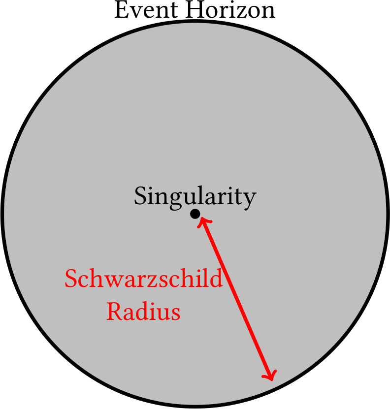
Figure 1: Artistic representation of a Schwarzschild black hole

Well, let’s discuss about the points where the Schwarzschild metric diverges. Looking at the radius term we see that, when \begin{equation} r = \frac{2 M G}{c^2} , \end{equation} the radius term diverges. When we have this value for the radius of the massive object we say that we are at the Schwarzschild radius and yeah, here comes the black holes. This value represents the event horizon for a black hole, in other words, the maximum distance that an external observer “can see”.

Black hole formation

We can say that black holes are formed due to the gravitational stellar collapse. Because a star is a “tug of war” between the pressure (due to the nuclear fusion of its components) and the gravitational force, when the second starts to win, the star starts to collapse, i.e., the nuclear power ends. Then, the star density increases a lot and, when decreasing more than its Schwarzschild radius, nothing more can escape: we have formed a black hole.

And what about the Schwarzschild metric? Well, it is the metric wich is able to describe de exterior of the star, turning to a black hole, when it is collapsing (let’s look at Birkhoff’s theorem, to know more).

Black hole types

And why the Schwarzschild black hole is the “first kind” of black holes? Because we can say that there are only four solutions for the Einstein’s equations describing the ones which are stationary and asimptotically planes (see more looking for the “no-hair” theorem):

• Schwarzschild black hole: characterized only by its mass $M$;
• Kerr black hole: characterized by its mass $M$ and angular momentum $L$;
• Reissner-Nordstrom black hole: characterized by its mass $M$ and its charge $Q$;
• Kerr-Newman black hole: characterized by its mass $M$, charge $Q$ and angular momentum $L$.

References

[1] J. B. Hartle, Gravity: an introduction to Einstein’s general relativity, Addison Wesley (San Francisco), 2003.

[2] J. Foster, J. D. Nightingale A Short Course in General Relativity, Springer Verlag (New York), 1994.