Graph Neural Networks

17 minute read

Published: December 01, 2023

Have you ever heard about graphs? What about graph neural networks (GNNs)? If you have never paid attention, let’s try to remind you that, structures like the image below are, actually, graphs. And they are filling all the internet.

Figure 1: A simple image background, that you can find anyplace in the internet.

Let’s go with me, to learn a bit about this amazing technique, able to tackle problems beyond the usual tabular data from the day-to-day to Cosmology!

This post can be followed in a Jupyter Notebook using my repo: https://github.com/natalidesanti/pytorch_and_GNNs. If you prefer (to not have headaches with installation dependencies) you can follow this on Google Colab:

Different data sets

Most of the time, we have a simple tabular data and we would like to make predictions given some columns (the input data) and other columns (the target data) of that table, which you would like to make some predictions using the input. This is the simplest idea behind “doing” traditional machine learning. This means that you will always have your input with the same shape, but a possible different number of samples.

The problem arises when you start looking for structured data. This means you can have different input data with different “number of objects” (what we will call, in the graph structure, as nodes). Also, you can include many other properties for these new entities. You can even think about it as a set of tables, each one with a different number of rows, to represent the different nodes per graph. This is the kind of data GNNs are amazing to deal with!

What is a graph?

Graphs are mathematical units represented by $3$ numbers: $G = G (n_i, e_{i j}, g)$:

$n_i$: node attributes (properties related to the objects translated into graphs)
$e_{i j}$: edge attributes (usually properties related to the two nodes in question)
$g$: global attribute (which represents the entire graph)

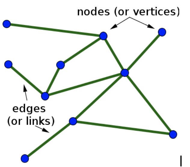
Figure 3: The idea of a graph - Image source: https://blog.fastforwardlabs.com/images/editor_uploads/2019-10-25-173715-graph_basics.png

(Almost) everything can be translated into a graph!

Let’s built the most simple graph ever: a graph with $3$ nodes: $[0, 1, 2]$, with node attributes $x_1 \in [-1, 0, 1]$ and $4$ edges (lines that take one node to another, as well theirs vice versa):

Figure 4: A simple graph, with all its information.

edge_index = torch.tensor([[0, 1], [1, 0], [1, 2], [2, 1]], dtype = torch.long) #Edge indexes
x = torch.tensor([[-1], [0], [1]], dtype = torch.float) #Node attributes
g = torch.tensor( [[3]], dtype = torch.int ) #Global attribute (number of nodes)
graph = Data(x = x, edge_index = edge_index.t().contiguous(), u = g)

To visualize it we can just use:

plt.figure(dpi = 100)
plt.title('Example of a graph colored by their node attribute')
G = to_networkx(graph, to_undirected = True)
nx.draw(G, node_color = graph.x[:, -1], node_size = 300, with_labels = True)

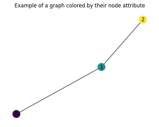
Figure 5: An example of what you will see with the piece of code - a graph, colored by their node information

A simple problem: predicting the center of mass of a box

In order for me, to explain how GNNs work, I will let you think about a simple problem with me. Imagine we need to compute the center of mass of some boxes, which contain some particles inside them.

Figure 6: Center of mass definition - Image source: https://studyingphysics.files.wordpress.com/2012/10/system-of-particles.jpg.

This means we will compute: $r_{CM} = \frac{ \sum_{i = 1}^{N} m_i r_{i} }{\sum_{i = 1}^{N} m_i }$.

For simplicity we can consider only particles of the same mass, distributed uniformly into a box of side $L$, with always the same number of particles. Then, we can generate the dataset using the following function:

def box_generator(NB, NP, L):

    #NB : number of boxes
    #NP : number of particles
    #L : size of the box
    #r : position of the particles [0, 1]
    #dist : distance of the particle in question with respect to the center of mass
    #cm : center of mass of each box

    r = {}
    cm = np.zeros((NB, 3))

    for i in range(NB):

        r[i] = np.random.uniform(low = 0.0, high = L , size = (NP, 3))
        cm[i] = np.average(r[i], axis = 0)

    return r, cm

To simplificate our task, let’s consider a box of side $L = 1.0$, $NP = 100$ particles per box (here, we could consider boxes with different number of particles per box – this will be left as an exercise for you guys), and $NB = 2000$ boxes. These boxes will look like the figure bellow:

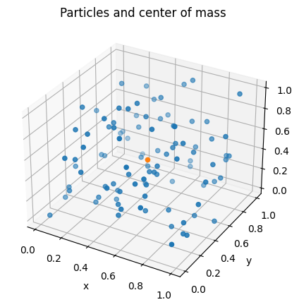
Figure 7: Visualization of one box, with particles and their center of mass.

Our task will be create a GNN to infer the $3$D value of the center of mass of each particle!

Creating the graphs

Now, with 2000 boxes at hand, we have a huge task to translate each one of them into a graph. That is why we will automatize this step. We can easily do this creating a routine which is responsible to read each one of the catalogs and create a graph for it. Then, the sequence of graphs can be arranged into a list and this will feed our GNN.

Creating the graph per se is a piece of art. Here I will show to you how to do this using kNN method. This means we will connect the particles in the box which are the $k$ neighbour of each other. This function will give to us the edges, i.e, what particles will be connected to each other. For simplicity, let’s choose $k = 10$. But, more than that, we have to choose the edge attributes. A simple choice is take their values as the modulus of the distance between the two particles in question. Then, I wrote this into two different functions:

To compute the edges:

def get_edges(pos, k_number):
  '''
  Compute knn graph and get edges and edge features
  '''
  # 1. Get edges
  edge_index = knn_graph(torch.tensor(pos, dtype = torch.float32), k = k_number, loop = False)

  # 2. Get edge attributes
  row, col = edge_index
  diff = pos[row] - pos[col]

  # Distance
  dist = np.linalg.norm(diff, axis = 1)

  edge_attr = np.concatenate([dist.reshape(-1, 1)])

  return edge_index, edge_attr

To create the graphs, choosing as node features the particle positions

def create_graphs(pos, NB):

    #Getting the edge indexes and edge attributes
    edges = {}
    edges_atrs = {}
    for i in range(NB):
        edges[i], edges_atrs[i] = get_edges_kNN(pos[i], 10)

    #Getting the node attributes
    x = {}
    for i in range(NB):
        x[i] = np.zeros( ( pos[i].shape[0], 3 ) )
    for i in range(NB):
      x[i][:, 0] = pos[i][:, 0]
      x[i][:, 1] = pos[i][:, 1]
      x[i][:, 2] = pos[i][:, 2]

    #Getting the target attributes
    y = np.zeros( (NB, 3) )
    for i in range(NB):
      y[i, :] = (CM[i, :] - mean)/std #Data pre-processing the target value

    dataset = []
    for i in range(NB):
        edge_index = torch.tensor(edges[i].T, dtype = torch.long)
        edge_atrs = torch.tensor(edges_atrs[i], dtype = torch.float)
        xs = torch.tensor(x[i], dtype = torch.float32)
        ys = np.reshape(y[i], (1, 3))
        data = Data(x = xs, edge_index = edge_index.t().contiguous(), edge_atrs = edge_atrs, y = ys)
        dataset.append(data)

    return dataset

In the function above you can notice I am using mean and std, which correspond to a data pre-procesing scheme to change the range of the values we wanna predict. This move is done in order to get a faster and better convergence of the machine learning methods, in general.

Which looks like:

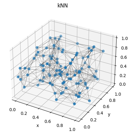
Figure 8: Visualization of one box, with their particles converted into a graph.

In order to get the dataset ready to use it into the GNN we need to convert it into tensors and split it into training, validation and testing subsets in the right structures. We can do so using the following function:

def transform_dataset(dataset, frac_train, frac_val, batch_size):
    '''
    frac_train: fraction of the dataset to use in the training
    frac_val:   fraction of the dataset to use in the validation
    batch_size: number of samples to work through before updating the internal model parameters
    '''

    #Getting the training, validation, and testing sets

    dataset_train = dataset[:int(len(dataset)*frac_train)]
    dataset_val = dataset[int(len(dataset)*frac_train):int(len(dataset)*(frac_train + frac_val))]
    dataset_test = dataset[int(len(dataset)*(frac_train + frac_val)):]

    #Organizing in batches
    train_loader = DataLoader(dataset = dataset_train, batch_size = batch_size)
    val_loader = DataLoader(dataset = dataset_val, batch_size = batch_size)
    test_loader = DataLoader(dataset = dataset_test, batch_size = batch_size)

    return train_loader, val_loader, test_loader

Graph Neural Networks (GNNs) ________

Now it is time to tell you something about the most interesting part, the GNNs. Graphs can be used to perform many different tasks. I really love the picture below, which represents many tasks graphs can be employed to.

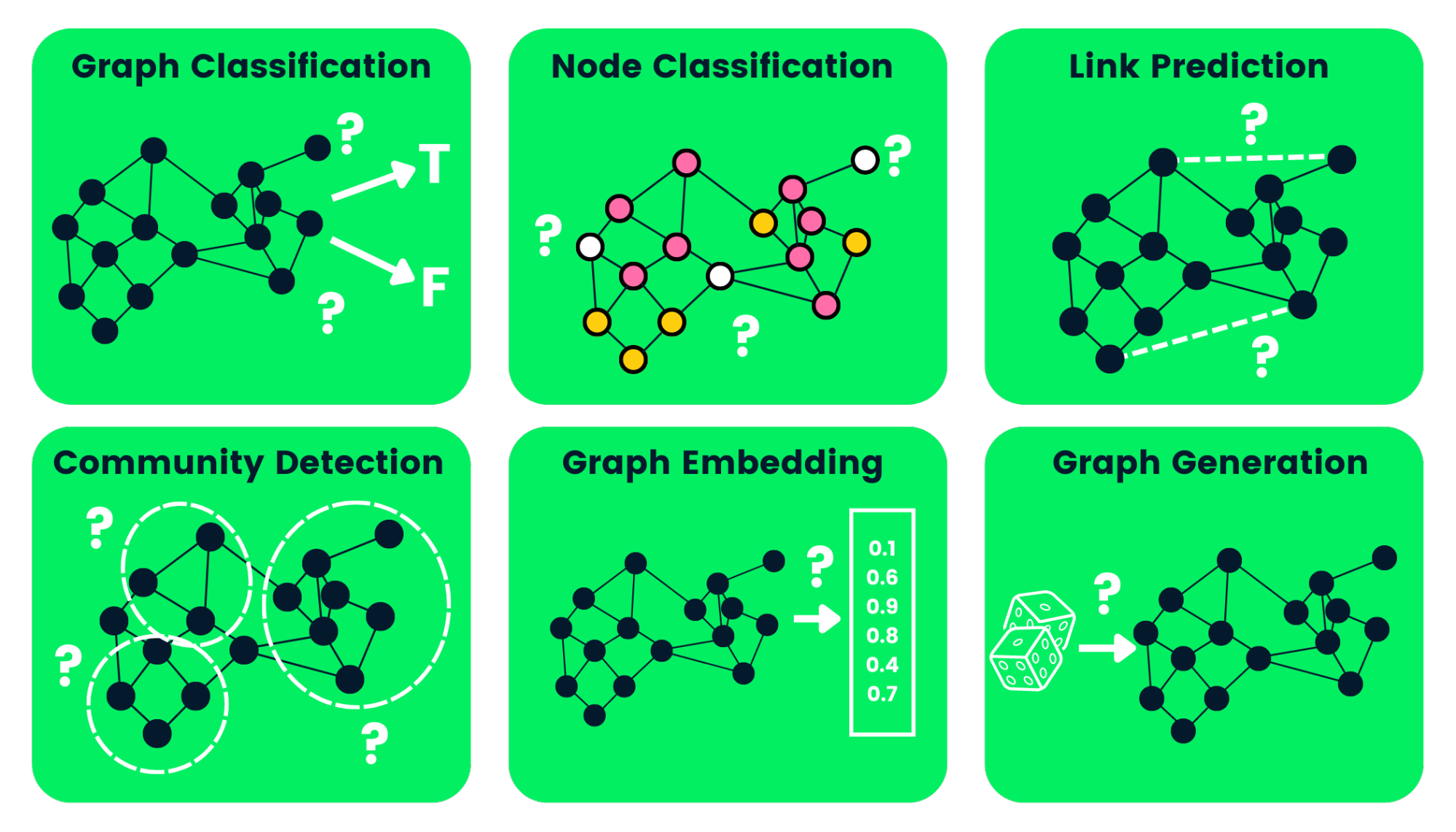
Figure 9: Graph tasks - Image source: https://images.datacamp.com/image/upload/v1658404112/Types_of_Graph_Neural_Networks_fd300394e8.png.

In this post I will present to you how to use graph embeding. This means we will predic a global property for each graph. We can do so using an amazing archtecture called message passing scheme where we are going to feed the GNN with the graphs and update the values of their nodes and edge attributes according to many layers/blocks without changing the shape of the graphs. This can be done using Metalayers and buiding a model to update the values of the node and edge attributes in the way we desire.

After the graph is completely updated we are responsible to transform it in a way to be able to solve the proposed task. Here we will solve a regression problem, i.e., we are going to compute one number for each graph. In this case we will compress the whole updated version of the graph into an awway and infer the center of mass.

Let’s describe the edge and node models:

Edge model:

$e_{i j}^{(\ell + 1)} = \mathcal{E}^{(\ell + 1)} \left( \left[ n_{i}^{(\ell)}, n_{j}^{(\ell)}, e_{i j}^{(\ell)} \right] \right)$,

where $\mathcal{E}^{(\ell + 1)}$ represents a MLP;

Node model:

$n_{i}^{(\ell + 1)} = \mathcal{N}^{(\ell + 1)} \left( \left[ n_{i}^{(\ell)}, \bigoplus_{j \in \mathfrak{ N}_i } e^{(\ell + 1)} i j \right] \right)$

where $\mathfrak{N}_i$ represents all neighbors of node $i$, $\mathcal{N}^{(\ell + 1)}$ is a NN, and $\oplus$ is a multi-pooling operation responsible to concatenate several permutation invariant operations. Several aggregators can enhance the expressiveness of GNN!

We can code the above lines writting a function for each model:

Edge model:

class EdgeModel(torch.nn.Module):

    def __init__(self, num_node_in, num_node_out, num_edge_in, num_edge_out,
                 hiddens):

        super().__init__()

        in_channels = ( 2 * num_node_in + num_edge_in) #Considering both nodes and the edge in question

        #MLP layer archtecture
        layers = [Linear(in_channels, hiddens),
                  LeakyReLU(0.2),
                  Linear(hiddens, num_edge_out)]

        #Defining the MLP
        self.edge_mlp = Sequential(*layers)

    def forward(self, src, dest, edge_atrs, u, batch):
      # src: source nodes
      # dst: destination nodes
      # edge_atrs: edge attributes
      # u: global properties

      #Updating the edges considering the nodes and edges
      out = torch.cat([src, dest, edge_atrs], dim = 1)

      #Applying the MLP
      out = self.edge_mlp(out)

      return out

Node model:

class NodeModel(torch.nn.Module):

    def __init__(self, num_node_in, num_node_out, num_edge_in, num_edge_out,
                 hiddens):

        super().__init__()

        in_channels = num_node_in + 3*num_edge_out #Considering the node in question and 3 pooling operations

        #MLP layer archtecture
        layers = [Linear(in_channels, hiddens),
                  LeakyReLU(0.2),
                  Linear(hiddens, num_node_out)]

        #Defining the MLP
        self.node_mlp = Sequential(*layers)

    def forward(self, x, edge_index, edge_atrs, u, batch):
        # x: node attributes
        # edge_index: edge indexes
        # edge_atrs: edge attributes
        # u: global property

        row, col = edge_index

        #The edge attributes
        out = edge_atrs

        #Multipooling the edge attributes
        out1 = scatter_add(out, col, dim = 0, dim_size = x.size(0))
        out2 = scatter_max(out, col, dim = 0, dim_size = x.size(0))[0]
        out3 = scatter_mean(out, col, dim = 0, dim_size = x.size(0))

        #Updating the node considering the node and the multipooling operation in the edges
        out = torch.cat([x, out1, out2, out3], dim = 1)

        #Applying the MLP
        out = self.node_mlp(out)

        return out

Notice that we have to define the GNN parameters to run these functions. Something like this:

num_node_in = 3 #We are working with 3 node attributes
num_node_out = 3 #We will compute the 3D center of mass

hiddens = 32 #Fixing the number of neurons per layer, just for simplicity

num_edge_in = 1 #Our number of edge attributes is only one (distance between nodes)
num_edge_out = 1 #Same

After defining these pieces of the model we can finally use them in the MetaLayer and define the whole model such as:

class GNN(torch.nn.Module):

  def __init__(self, node_features, n_layers, hidden_channels, global_out):

    super().__init__()

    self.n_layers = n_layers #Defining the number of Metalayers
    self.global_out = global_out #Defining the dimension of the final output

    num_node_in = node_features #Defining the number of input node features
    num_node_out = num_node_in #Defining the number of output node features

    num_edge_in = 1 #Defining the number of input edge features
    num_edge_out = num_edge_in #Defining the number of output edge features

    layers = []

    #Defining the first MetaLayer: with the node and edge models
    inlayer = MetaLayer(edge_model = EdgeModel(num_node_in, num_node_out,
                                               num_edge_in, num_edge_out,
                                               hidden_channels),
                         node_model = NodeModel(num_node_in, num_node_out,
                                                num_edge_in, num_edge_out,
                                                hidden_channels)
                         )

    layers.append(inlayer)

    num_node_in = num_node_out
    num_edge_in = num_edge_out

    #Defining the inner MetaLayers: with the node and edge models - the hidden graph blocks
    for i in range(self.n_layers - 1):

      layer_hidden = MetaLayer(edge_model = EdgeModel(num_node_in, num_node_out,
                                                      num_edge_in, num_edge_out,
                                                      hidden_channels),
                              node_model = NodeModel(num_node_in, num_node_out,
                                                     num_edge_in, num_edge_out,
                                                     hidden_channels)
                              )
      layers.append(layer_hidden)

    self.layers = ModuleList(layers)

    #Defining the MLP for the compressed version of the graph
    self.final_out_layer = Sequential(
                                      Linear(3*num_node_out, hidden_channels),
                                      LeakyReLU(0.2),
                                      Linear(hidden_channels, hidden_channels),
                                      LeakyReLU(0.2),
                                      Linear(hidden_channels, hidden_channels),
                                      LeakyReLU(0.2),
                                      Linear(hidden_channels, self.global_out)
                                      )

  def forward(self, data):

    x, edge_index, edge_atrs, batch = data.x, data.edge_index, data.edge_atrs, data.batch

    #Message passing
    for layer in self.layers:
      x, edge_atrs, _ = layer(x, edge_index, edge_atrs, None, data.batch)

    #Multipooling all the nodes
    addpool = global_add_pool(x, batch)
    maxpool = global_max_pool(x, batch)
    meanpool = global_mean_pool(x, batch)

    #Concatenating the compressed version of the graph
    out = torch.cat( [ addpool, maxpool, meanpool], dim = 1 )

    #Final linear layer
    out = self.final_out_layer(out)

    return out

The model is finally ready:

model = GNN(node_features = num_node_in, n_layers = 2, hidden_channels = hiddens, global_out = 3).to(device)

Now, we just need to train it:

loss_fn = torch.nn.MSELoss()
optimizer = torch.optim.Adam(model.parameters(), lr = 5e-3, weight_decay = 1e-6)

epochs = 200

lloss_train = []
lloss_val = []

print("Starting training...")

for i in range(epochs):

    model.train()  #Telling the model we are training :p
    aux_train = 0
    for data in train_loader:
        data = data.to(device)
        out = model(data)
        loss = loss_fn(out, torch.from_numpy( np.array(data.y)[:, 0] ).float().to(device) )
        optimizer.zero_grad()
        loss.backward()
        optimizer.step()
        aux_train += loss.item()
    lloss_train.append( aux_train/len(train_loader) )

    if i % 20 == 0:
        print(f"Epoch {i} | Train Loss {aux_train/len(train_loader)}")

    model.eval() #Telling the model we are testing :p
    aux_val = 0
    for data in val_loader:
        data = data.to(device)
        out = model(data)
        loss = loss_fn(out, torch.from_numpy( np.array(data.y)[:, 0] ).float().to(device) )
        aux_val += loss.item()
    lloss_val.append( aux_val/len(val_loader) )

    if i % 20 == 0:
        print(f"Epoch {i} | Train Loss {aux_val/len(val_loader)}")

After we have trained the model we can infer ofer the test set using:

lloss_test = []
preds = []
yss = []
for data in test_loader:
  out = model(data.to(device))
  preds.append( out.detach().cpu().numpy() )
  yss.append( np.array(data.y) )
  loss = loss_fn(out, torch.from_numpy( np.array(data.y)[:, 0] ).float().to(device) )
lloss_test.append( loss.data.cpu().numpy() )
loss_test = np.mean(lloss_test)
loss_test

Then, we can see if everything is all right just making some plots regarding the histogram of the predicted versus true values or the famous truth $\times$ predictions plots too.

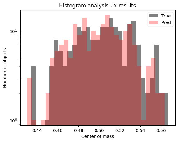
Figure 10: Histogram showing predicted values for the test set of $x$ component of center of mass.

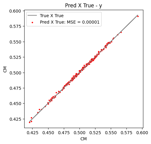
Figure 11: Truth $\times$ predicted values for the test set of $y$ component of center of mass.

In this post we followed a simple example to illustrate how we can use graphs. I hope you have enjoyed and that now you will be inspired to start working on GNNs. See you next time!

Supplementary material

If you wanna learn more about GNNs you can check amazing materials as the ones listed below:

You can see amazing scientific publications using GNNs such as:

Massara, E., Villaescusa-Navarro, F., & Percival, W. J. 2023, arXiv e-prints, arXiv: 2309.05850;
de Santi, N. S. M., Shao, H., Villaescusa-Navarro, F., et al. 2023, ApJ, 952, 69, doi: 10.3847/1538-4357/acd1e2;
Chen, Z., Mao, H., Li, H., et al. 2023, arXiv: 2307.03393;
Shao, H., de Santi, N. S. M., Villaescusa-Navarro, F., et al. 2023, arXiv e-prints, arXiv: 2302.14591;
Villanueva-Domingo, P., & Villaescusa-Navarro, F. 2022, ApJ, 937, 115, doi: 10.3847/1538-4357/ac8930;
Shao, H., Villaescusa-Navarro, F., Villanueva-Domingo, P., et al. 2022b, arXiv e-prints, arXiv: 2209.06843;
Villanueva-Domingo, P., Villaescusa-Navarro, F., Genel, S., et al. 2021, arXiv: 2111.14874;
Villanueva-Domingo, P., Villaescusa-Navarro, F., Anglés-Alcázar, D., et al. 2022, ApJ, 935, 30. doi: 10.3847/1538-4357/ac7aa3;
Makinen, T. L., Charnock, T., Lemos, P., et al. 2022, arXiv e-prints, arXiv: (2207.05202)[https://arxiv.org/abs/2207.05202];
Anagnostidis, S., Thomsen, A., Kacprzak, T., et al. 2022, arXiv e-prints, arXiv: (2211.12346)[https://arxiv.org/abs/2211.12346];
Wang, N., Zhang, Y., Li, Z., et al. 2018, arXiv e-prints, arXiv: 1804.01654.

Share on

Twitter Facebook LinkedIn

Natalí de Santi