Casimir effect

In this post you will see what is the bizarre Casimir Effect. I will start telling you about quantum fluctuations, give you some qualitative definition of it and, then, two quantitative descriptions. As I warned you in the previous post (Harmonic Oscillator), the Physics/Mathematics behind of this effect are the quantum harmonic oscillators!

What are Quantum Fluctuations? And what heck is the quantum vacuum?

In Classical Mechanics the evolution of a system of particles is given knowing the initial position $x$ and the momentum $p$ of all particles, as well the forces applied on them. But, this way of “thinking” about the description changes a lot when we go to Quantum Mechanics, due the Uncertainty Principle (of Heisenberg). This principle could be expressed using two equations \begin{equation} \Delta x \cdot \Delta p \gtrsim \hbar/2 , \end{equation} \begin{equation} \Delta E \cdot \Delta t \gtrsim \hbar/2 . \end{equation} The first equation says that we cannot determine, with precision and at the same time, the position and momentum of some particle. The second one implies that a perfect measure of the energy of some system needs an infinite time.

A really interesting consequence of this principle is that we can violate momentously the conservation energy principle if and just if this happens by an interval of time very small, lower than $\hbar/(2 \Delta E)$. Here we have the energy quantum fluctuations! Then, using the energy-mass relation \begin{equation} E = m c^2 \end{equation} we can interpret the quantum fluctuations of energy, for instance, in the vacuum, as virtual particles. Because those particles live just by an infinitesimal amount of time we cannot detect them. Although, we can “see” the effects generated by their existence. Due to them, we have the mediation of fundamental interactions (like the strong iteraction or even the virtual photons, in the electrical force) [1].

Ok, but why the title of this section contains the quantum vacuum? To be clear, everything! So, every time that we think about vacuum we imagine a physical region obtained excluding every kind of matter on it, right? However, the entity quantum vacuum is a vacuum populated by a legion of particles, yeah, the virtual particles, that could not be removed. And, of course, they exists due the quantum fluctuations!

The Casimir effect - Qualitative explanation

The vacuum quantum fluctuations are responsible to generate the bizarre Casimir effect. In this phenomenon, there is the attraction between two metallic plates, that are electrically neutral and with negligible mass.

Figure 1: Artistic representation of Casimir effect

More specifically, the vacuum quantum fluctuations generates a difference of pressure between the plates and in its exterior. More specifically, due to the lower amount of space between the plates, the density of virtual particles there is lower than in the exterior space. Thus, as we have a huge pressure outside, the plates attracts to each other.

In fact, any medium supporting oscillations can be an analogous to the Casimir effect. But, a classical analogue to this effect (that I really love) is the attraction between two metal and electrically neutral plates, in some liquid, with sonication machines. In the video Water Wave Analog of the Casimir Effect, we have the demonstration of it. The video shows that traveling water waves carry momentum! There is a container of liquid (ethyl alcohol) with a dye fluorescent (so, the waves can be seen) and two parallel plates are suspended from clamps attached to a support. The container rests on a shaker. The shaker is driven with noise in a band of frequencies from 10 to 20 Hz, and excites surface waves. Therefore, the plates attract to each other. Another very interesting reference is given by the paper.

A really briefly history, Quantum Field Theory and the problem with infinities

In 1948 Hendrik Brugt Gerhard Casimir proposed a way to perturb the vacuum and achieve a finite variation of energy $\Delta E$, which was known as Casimir effect. To understand this phenomenon, quantitatively speaking, you need to understand a little of Quantum Field Theory (QFT), which states that all of the various fundamental fields, such as the electromagnetic field or the Klein-Gordon field, must be quantized at each and every point in space. In other words, the field is a function of the time and space. Vibrations in this field propagate and are governed by the appropriate wave equation for the particular field in question. At the “most basic level”, the field at each point in space is a simple harmonic oscillator, and its quantization “places” a quantum harmonic oscillator at each point. That is why I started to study harmonic oscillator!!!

So, in order to understand where and why the Casimir effect arises, let’s start with the Klein-Gordon field, the most basic field in QFT.

The Klein-Gordon field

The Klein-Gordon equation is a relativistic wave equation, related to the Schrodinger equation (yeah, the most famous equation of the Quantum Mechanics!). This wave equation \begin{equation} \left[ \frac{1}{c^2} \frac{\partial^2}{\partial t^2} - \nabla^2 + \frac{m^2 c^2}{\hbar} \right] \phi (x) = 0 \end{equation} describes a scalar field of mass $m$ and spin 0. This equation could be obtained from the Hamiltonian density \begin{equation} \mathcal{H} = \frac{1}{2} \left[ \pi (x)^2 + |\nabla \phi|^2 + \mu^2 \phi(x)^2 \right], \end{equation} where \begin{equation} \pi(x) = \frac{\partial \mathcal{L}}{\partial \dot{\phi}} = \frac{1}{c^2} \dot{\phi}(x) \end{equation} is the conjugate momentum to the field $\phi(x,t)$ and $\mu = m c / \hbar$.

The quantum version of this field could be obtained imposing the commutation relations \begin{equation} \left[\hat{\phi}({\bf x},t), \dot{\hat{\phi}}({\bf x}’,t) \right] = i \hbar c^2 \delta({\bf x} - {\bf x}’) \end{equation}
\begin{equation} \left[\hat{\phi}({\bf x},t), \hat{\phi}({\bf x}’,t) \right] = \left[ \dot{\hat{\phi}}({\bf x},t), \dot{\hat{\phi}}({\bf x}’,t)\right] = 0. \end{equation} To interpret this, we can expand the Klein-Gordon field in \begin{equation} \hat{\phi} (x) = \hat{\phi}^+ (x) + \hat{\phi}^- (x), \end{equation} using \begin{equation} \hat{\phi}^+ (x) = \sum_k \left( \frac{\hbar c^2}{2V\omega_k}\right)^{1/2} \hat{a}({\bf k}) e^{-ikx} \end{equation} and \begin{equation} \hat{\phi}^- (x) = \sum_k \left( \frac{\hbar c^2}{2V \omega_k}\right)^{1/2} \hat{a}^{\dagger}({\bf k}) e^{ikx}. \end{equation} Here, $V$ is the volume of a cube with side $L$ ($V = L^3$), $\omega_k$ is the angular frequency of oscillation and $\mathbf{k}$ is the wave vector. Besides, the sum is over all the allowed $\mathbf{k}$s and \begin{equation} k^0 = \frac{1}{c} \omega_k = + \left( \mu^2 + {\bf k}^2 \right)^{1/2}. \end{equation} The, $k$ is the quadrivector of a particle of mass $m = \mu \hbar/c$, momentum $\hbar \mathbf{k}$ and energy \begin{equation} E = \hbar\omega_k = + \sqrt{m^2c^4 + c^2(\hbar{\bf k})^2}. \end{equation} Using the expansion of the Klein-Gordon field and the commutation relation (for its quantization) we can obtain the commutation relations between the operator $\hat{a}({\bf k})$ and $\hat{a}^{\dagger}({\bf k})$, which are \begin{equation} \left[ \hat{a}({\bf k}), \hat{a}^{\dagger}({\bf k}’) \right] = \delta_{\bf k, k’}
\end{equation} \begin{equation} \left[ \hat{a}({\bf k}), \hat{a}({\bf k}’) \right] = \left[ \hat{a}^{\dagger}({\bf k}), \hat{a}^{\dagger}({\bf k}’)\right] = 0 . \end{equation} If you remember (or can remember here), it is exactly the quantum harmonic oscillator commutation relations of the raise and low operators!

At the same time, we can rewrite the Hamiltonian using these operators as \begin{equation} H = \sum_{k} \hbar \omega_k \left[ a^{\dagger}({\bf k})a({\bf k}) + \frac{1}{2} \right]. \end{equation} Paying attention on this Hamiltonian you can see that the system is described by a set of decoupled harmonic oscillators! Moreover, the state of lower energy, i.e., the vacuum state $\langle 0 \rangle$ is \begin{equation} a({\bf k}) \left|0\right> = 0, \hspace{0.6cm}\forall {\bf k}, \end{equation} or, equivalently, as \begin{equation} \phi^+ (x) \left|0\right> = 0, \hspace{0.6cm} \forall x. \end{equation} Therefore, the vacuum has infinity energy \begin{equation} E_0 = \frac{1}{2}\sum_{k}\hbar\omega_k . \end{equation} In fact, this summation includes a infinity number of normal modes $k$ and the frequency $\omega_k$ increases with it. However, this is a problem only when we wanna look exactly at this term, because, in all physical measures, as we only measure difference of energies, it is automatically removed!

In QFT, this kind of infinities arises all the time: not only for the Klein-Gordon field, but, for instance, for the electromagnetic field too (because all the fields could be seen as a set of quantum harmonic oscillators!). To understand what to do with these quantities, there is something called renormalization, a collection of techniques to treat infinities. Inside it, there is the regularization methods, which is a way to mathematically define the divergences, using theory of limits. Here I will tell you two techniques of it:

• Cut-off regularization,
• Dimensional regularization.

And, the reason why I will do this is that, treating the infinity for the vacuum, we are computing a finite value for it $\Rightarrow$ deducing the Casimir effect.

Approach 1: Cut-off regularization

In the zero-point energy of the electromagnetic field, there is a term of the frequencies $\omega_k$. This term depend on the geometry of the volume in which the field is confined. If the geometrical form changes the frequency of the normal modes, the zero-point energy will also change [2].

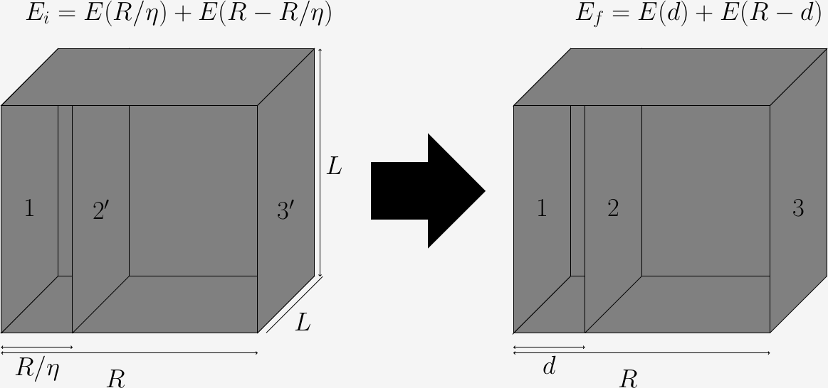
Figure 2: Casimir effect for cut-off regularization

Here, we can consider the region contained in a closed metallic box, electrically neutral of length $R$ and basal area $A = L^2$. Inside this box we introduce another plate, at some distance from the first one (initially it is at a distance $d$ and at the final position it is at a distance $R/\eta$). We are interested in the energy of the system depending on the position of one of the plates. And, to compute that energy, subtract the energy of a final ($f$) from an initial configuration ($i$): \begin{equation} U (d, R, A) = E_i - E_f = [E (R/\eta) + E (R - R/\eta)] - [E (d) + E (R - d)] . \end{equation} To implies in the Casimir Effect we need to move the walls, in the way that the quantization volume becomes infinity. Thus, we are computing \begin{equation} U (d, A) = \lim_{R \rightarrow \infty} U (d, R, A). \end{equation} As every piece of that energy diverges, we need to find a cut-off.

This cut-off could be made using a cut-off parameter, that could be the wavelength $\lambda$. Then, the vacuum energy could be written as \begin{equation} E = \frac{\hbar}{2} \sum_{k} \omega_k e^{- \lambda \omega_k/c}. \end{equation} In the case of a box, the frequency is \begin{equation} \label{k} \omega_{l,m,n} = c\hspace{0.1cm}k_{l,m,n} (d, L, L) = c\hspace{0.1cm} \sqrt{\left(\frac{l\pi}{d}\right)^2 + \left(\frac{m\pi}{L}\right)^2 + \left(\frac{n\pi}{L}\right)^2} \hspace{0.2cm}, \end{equation} where $l, m, n \in \mathbb{N}$. Therefore, the energy (just disconsidering a factor of $\hbar c/2$) becomes \begin{equation} E (d, L) = \sum_{l, m, n = 0}^{\infty} k_{l, m, n} (d, L, L) \hspace{0.1cm}e^{- \lambda k_{l, m, n} (d, L, L)} \hspace{0.2cm}. \label{E0} \end{equation} In the limit that we want ($L \gg d$), the energy becomes \begin{equation} E (d, L) = \frac{A \pi^2}{2d} \frac{d^2}{d\alpha^2} \left[ \sum^{\infty}{n=0} \frac{B_n}{n!} \left(\frac{\alpha}{d}\right)^{n-2}\right] \hspace{0.2cm}, \end{equation} where $\alpha = \pi \lambda$ and the coefficients $B_n$ are the _Bernoulli’s numbers. In the limit where $\alpha \rightarrow 0$, we could keep just the firsts terms of this expression, i.e., \begin{equation} E (d, L) = \frac{A \pi^2}{2} \frac{d^2}{d\alpha^2} \left[\frac{d}{\alpha^2} - \frac{1}{2\alpha} + \frac{1}{12d} - \frac{\alpha^2}{720d^3} + O(\alpha^4) \right] \hspace{0.2cm}. \end{equation}

In the case of the difference of energy $U (d, A)$, the terms proportionals to $\alpha^{- 2}$ and $\alpha^{- 1}$ cancel out. Moreover, the terms of order $\alpha^0$ are zero because the derivative operation. In this way, we got \begin{equation} U (d, A) = -\frac{A \pi^2 \hbar c}{720} \lim_{R \rightarrow \infty} \lim_{\alpha \rightarrow 0} \left{ \left[\frac{1}{d^3} + \frac{1}{(R-d)^3}

• \frac{1}{(R/\eta)^3} - \frac{1}{(R - R/\eta)^3}\right] \right} \end{equation} and finally \begin{equation} \label{UUU} U(d,A) = -\frac{A \pi^2}{720} \, \frac{\hbar c}{d^3} \hspace{0.2cm}. \end{equation}

If we compute the force between the plates, we obtain \begin{equation} \label{F} F = -\frac{\partial}{\partial d} \hspace{0.1cm} U(d,A) = - \frac{A \pi^2}{240} \, \frac{\hbar c}{d^4} \hspace{0.2cm}, \end{equation} which is an attractive force.

Approach 2: Dimensional regularization

In the case of the dimensional regularization we can consider two metal, neutral metallic plates in the vacuum, separated by a distance $d$ [3].

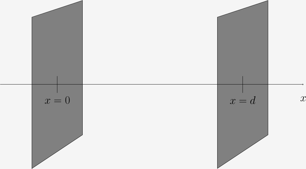
Figure 3: Casimir effect for dimensional regularization

This geometry allows the frequency $\omega_k$ be written as \begin{equation} \omega_{k, n} = c\hspace{0.1cm}\sqrt{k^2 + \left(\frac{n\pi}{d}\right)^2} \hspace{0.2cm}, \end{equation} where $n$ represents the longitudinal mode of oscillation and $k$ represents the transversal wave vector. The energy is given by unit of area (because we are in one dimension, at least until now) by \begin{equation} \label{RN} E = \frac{\hbar c}{2} \sum_{n = 1}^{\infty} \int^{\infty}{- \infty} \frac{d^2k}{(2\pi)^2} \sqrt{k^2 + \left(\frac{n\pi}{d}\right)^2} \hspace{0.2cm}. \end{equation} To apply the _dimensional regularization we can fix the transversal dimension equal to $D$ and, we need to chance the dimension of the square root for $s$, i.e., we write \begin{equation} \label{RN1} E = \frac{\hbar c}{2} \sum_{n = 1}^{\infty} \int \frac{d^D k}{(2 \pi)^D} \left[ k^2 + \left(\frac{n \pi}{d}\right)^2 \right]^{- s}\hspace{0.2cm}. \end{equation} Clearly, at the end of this computations, we need to take the limit where $D \rightarrow 2$ and $s \rightarrow - 1/2$. Using properties from the special functions Gamma $\Gamma (z)$ and Riemmann’s zeta $\zeta(z)$, like \begin{equation} \int^{\infty}{- \infty} \frac{d^D k}{(2 \pi)^D} \left[ k^2 + \left(\frac{n \pi}{d}\right)^2 \right]^{- s} = \frac{1}{\Gamma (s)} \int^{\infty}{- \infty} \frac{d^D k}{(2 \pi)^D} \int^{\infty}{0} d\tau \hspace{0.2cm} \tau^{s - 1} \hspace{0.2cm} e^{- \tau \left[ k^2 + (n\pi/d)^2 \right]}\hspace{0.2cm}, \end{equation} which is valid for $s > 0$ but not for $s = - 1/2$. So, why we can use it? Because we can write the energy as \begin{equation} \label{EEE} E = \frac{\hbar c}{\Gamma (s)}\hspace{0.2cm} \frac{\Gamma (s - D/2)}{2^{D + 1} \pi^{2s - D/2}} \hspace{0.2cm} d^{2s - D} \hspace{0.2cm}\zeta (2s - D) \hspace{0.2cm}. \end{equation} Of course this expression is undetermined for $2s - D \leq 1$, but, using the _reflection property \begin{equation} \Gamma \left(\frac{z}{2}\right)\hspace{0.2cm}\zeta(z)\hspace{0.2cm}\pi^{- z/2} = \Gamma \left(\frac{1 - z}{2}\right)\hspace{0.2cm}\zeta(1 - z) \hspace{0.2cm}\pi^{(z-1)/2} \end{equation} with $z = 2s - D$, we obtain \begin{equation} \label{Efinal} E = \frac{\hbar c}{\Gamma(s)}\hspace{0.2cm}\frac{\pi^{-(D + 1)/2}}{2^{D + 1}} \hspace{0.2cm}d^{2s - D}\hspace{0.2cm}\Gamma \left( \frac{1 - 2s + D}{2} \right)\hspace{0.2cm}\zeta \left(1 - 2s + D\right) \hspace{0.2cm}. \end{equation} The above result is well behaved when we take the physical limits $s \rightarrow - 1/2$ and $D \rightarrow 2$. Then, using that $\Gamma(-1/2) = - 2 \sqrt{\pi}$ and $\Gamma(2) = 1$ e $\zeta(4) = \pi^4/90$, the energy $U(d)$, between the two plates at a distance $d$ from each other, is given by \begin{equation} U (d) = 2 \hspace{0.2cm}\lim_{s \rightarrow -1/2} \hspace{0.2cm} \lim_{D \rightarrow 2} E = 2 \hspace{0.2cm} \frac{\hbar c}{\Gamma(-1/2)} \hspace{0.2cm}\frac{\pi^{- 3/2}}{2^3 d^3} \hspace{0.2cm}\Gamma(2) \hspace{0.2cm}\zeta(4) = - \hspace{0.2cm}\frac{\pi^2}{720} \hspace{0.2cm}\frac{\hbar c}{d^3} \hspace{0.2cm}. \end{equation} Remember that this results is multiplied by $2$ because the photons have two polarization states.

Therefore, the force (per unit of area) is \begin{equation} \label{F2} F(d) = - \frac{\partial}{\partial d} U(d) = - \frac{\pi^2}{240} \frac{\hbar c}{d^4}\hspace{0.2cm}, \end{equation} which is in accordance with the result from the approach 1. This method could be seen as “pure mathematical magic”, but it is “more robust”, when compared with the previous one, in the sense that it method does not need any subtraction of energy on its deduction.

Conclusions

Both approaches makes clear that the force between two metallic and uncharged plates, in other words, the Casimir effect, depends of $\hbar$ and $c$, showing the pure quantum nature behind this effect.

References

[1] David Griffiths, Introduction to Elementary Particles, John Wiley & Sons, 2012.

[2] W. Greiner, Quantum Mechanics - Special Chapters, Springer (Frankfurt), 2001.

[3] K. A. Milton, The Casimir Effect - Physical Manifestation of Zero-Point Energy, World Scientific (Singapura), 2001.