
Pytorch
Published:
Hello there! If you just came to this blog and you would like to learn something about PyTorch I believe you can find something to start playing around. In this post we will see how to write a simple code to solve a simple regression problem. This means we will do predictions for a quantity $y$, given values for their predictor (the input) $x$ for a noised: $y = a x + b$.
The first warn is that you can follow this post on Google Colab: ![]() . If you prefer to download it as a
. If you prefer to download it as a Jupyter Notebook and run on your own machine, please, go to the repo: pytorch_and_GNNs.
The first thing we could do is to learn that it is faster to run codes on the GPUs. That is why we have to define the processing unit and transfer our data and our model to there:
device = torch.device("cuda:0" if torch.cuda.is_available() else "cpu")
After defining the unit to process everything it is time to create the data set:
#Create Dataset
def generate_data(a, b, num_examples):
    '''
    Generate y = a x + b + noise
    '''

    x = np.random.uniform(0, 1, num_examples)
    y = a*x + b
    y += np.random.normal(0, 0.05, num_examples)

    df = pd.DataFrame(data = np.array([x, y]).T, columns = ['x', 'y'])

    return df
Then, the generated data will look like this:
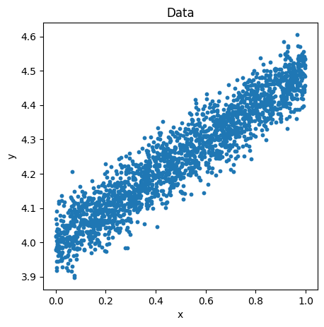
Figure 1: Generated data set.
Then, in this tutorial we are going to: ${x} \Rightarrow {y}$, using a simple Neural Network in Pytorch.
Transforming the dataset
First, we need to convert the data set in $3$ fractions:
- Train
- Validation
- Test
Second, we need to transform the data set using: $x \Rightarrow \frac{(x - x_{mean})}{x_{std}}$ and $y \Rightarrow \frac{(y - y_{min})}{(y_{max} - y_{min})}$. This is done to constrain the range of all the input variables ($x$, $y$) to small and similar values to get a faster convergence of the method.
Third, we need to convert the data into something to be understandable by PyTorch. We convert the data into tensors, then, in TensorDataSet, and DataLoader. This last step split one more time the sets using batches (number of samples to work through before updating the internal model parameters).
def transform_dataset(df, frac_train, frac_val, batch_size):
    '''
    frac_train: fraction of the dataset to use in the training
    frac_val:   fraction of the dataset to use in the validation
    batch_size: number of samples to work through before updating the internal model parameters
    '''

    #Randomizing the dataset
    df = df.sample(frac = 1)

    #Getting the training, validation, and testing sets
    x_train = np.array( [ df['x'].iloc[:int(df.shape[0]*frac_train)] ] ).T
    y_train = np.array( [ df['y'].iloc[:int(df.shape[0]*frac_train)] ] ).T

    x_val = np.array( [ df['x'].iloc[int(df.shape[0]*frac_train):int(df.shape[0]*(frac_train + frac_val))] ] ).T
    y_val = np.array( [ df['y'].iloc[int(df.shape[0]*frac_train):int(df.shape[0]*(frac_train + frac_val))] ] ).T

    x_test = np.array( [ df['x'].iloc[int(df.shape[0]*(frac_train + frac_val)):] ] ).T
    y_test = np.array( [ df['y'].iloc[int(df.shape[0]*(frac_train + frac_val)):] ] ).T

    #Getting the statistics from the training set
    mean = np.mean(x_train, axis = 0)
    std = np.std(x_train, axis = 0)
    min = np.mean(y_train, axis = 0)
    max = np.std(y_train, axis = 0)

    #Tranforming the training set
    x_train = (x_train - mean)/std
    x_val = (x_val - mean)/std
    x_test = (x_test - mean)/std

    y_train = (y_train - min)/(max - min)
    y_val = (y_val - min)/(max - min)
    y_test = (y_test - min)/(max - min)

    #Converting to torch reshaping
    x_train = torch.from_numpy(x_train.reshape(-1, 1)).float()
    y_train = torch.from_numpy(y_train.reshape(-1, 1)).float()

    x_val = torch.from_numpy(x_val.reshape(-1, 1)).float()
    y_val = torch.from_numpy(y_val.reshape(-1, 1)).float()

    x_test = torch.from_numpy(x_test.reshape(-1, 1)).float()
    y_test = torch.from_numpy(y_test.reshape(-1, 1)).float()

    #Converting to tensor dataset
    dataset_train = TensorDataset(x_train, y_train)
    dataset_val = TensorDataset(x_val, y_val)
    dataset_test = TensorDataset(x_test, y_test)

    #Organizing in batches
    train_loader = DataLoader(dataset = dataset_train, batch_size = batch_size)
    val_loader = DataLoader(dataset = dataset_val, batch_size = batch_size)
    test_loader = DataLoader(dataset = dataset_test, batch_size = batch_size)

    return train_loader, val_loader, test_loader, mean, std, max, min
Defining the Neural Network
A neural network is a collection of nodes (neurons) that are arranged in a series of layers:

Figure 2: Scheme representation of a NN. Image source: https://www.tibco.com/sites/tibco/files/media_entity/2021-05/neutral-network-diagram.svg]
Each connection has a weight, $\omega_i a_i$, and each layer is a summarization of them, plus a bias $b$, according to: \begin{equation} b_{\mu} + \sum_{\nu} W_{\mu \nu} a_{\nu} . \end{equation}
Another numeric transformation called activation function is responsible for performing a non linear transformation of the values of each layer \begin{equation} y_{\mu} = f \left( b_{\mu} + \sum_{\nu} W_{\mu \nu} a_{\nu} \right) , \end{equation} This activation function can assume different forms:
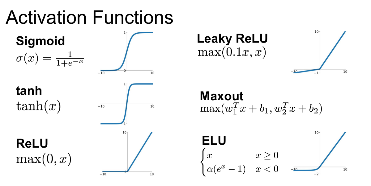
Figure 3: Examples of activation function. Image source: [https://miro.medium.com/max/1200/1ZafDv3VUm60Eh10OeJu1vw.png](https://miro.medium.com/max/1200/1ZafDv3VUm60Eh10OeJu1vw.png)
During the training process these weights are adjusted through the optimizer in epochs in order to minimize the difference between the network predictions $y_{pred}$, and the target values $y_{target}$ through the minimization of a loss function (that also can assume different forms). In this tutorial we are going to use the Mean Squared Error (MSE) \begin{equation} MSE = \frac{1}{m} \sum_{i = 1}^m (y_{pred} - y_{target})^2 . \end{equation}
Then, we can define the model such as:
class model(nn.Module):
  def __init__(self):

    super(model, self).__init__() #Initiating the model

    #Defining the linear layers and activation function
    self.layer1 = nn.Linear(1, 8)
    self.layer2 = nn.Linear(8, 16)
    self.layer3 = nn.Linear(16, 1)
    self.ReLU = nn.ReLU()

  #Forward pass
  def forward(self, x):
    '''
    Define the architecture at the same time as compute y
    '''
    x = self.ReLU(self.layer1(x))
    x = self.ReLU(self.layer2(x))
    y = self.layer3(x)

    return y
And the loss function and optimizer:
optimizer = torch.optim.Adam(model.parameters())
loss_func = torch.nn.MSELoss()
Training and validating the model
Now, it is time to do the magic:
epochs = 200 #Number of steps to train the model

lloss_train = []
lloss_val = []
for i in range(epochs):
  aux_train = 0
  model.train()  #Telling the model we are training :p
  for x, y in train_loader:
    x = x.to(device)
    y = y.to(device)
    prediction = model(x)
    tloss = loss_func(prediction, y)
    optimizer.zero_grad() #set the gradients to zero before starting to do backpropagation (i.e., updating the weights and biases)
    tloss.backward() #calculate the gradient during the backward pass in the neural network
    optimizer.step() #performs a single optimization step (parameter update)
    aux_train += tloss.item()
  lloss_train.append( aux_train/len(train_loader) )
  if i % 10 == 0:
    print(f"Epoch {i} | Train Loss {aux_train/len(train_loader)}")

  aux_val = 0
  model.eval() #Telling the model we are testing :p
  for x, y in val_loader:
    x = x.to(device)
    y = y.to(device)
    prediction = model(x)
    vloss = loss_func(prediction, y)
    aux_val += vloss.item()
  lloss_val.append( aux_val/len(val_loader) )
  if i % 10 == 0:
    print(f"Epoch {i} | Val Loss {aux_val/len(val_loader)}")
Notice that we are always passing the objects of the code to device, in order to do everything on the GPU.
One important practice after training the model is to analyse if it is ok, i.e., if we do not have a biased model that is:
- Overting: when the model gives accurate predictions for training data but not for new data (validation or test data). This can be seen when the validation loss is increasing or ir is higher while compared to the training loss.
- Underfitting: when the model is unable to capture the relationship between the input and output variables accurately. This can be seen when the validation loss is decreasing of it is lower than the training loss.
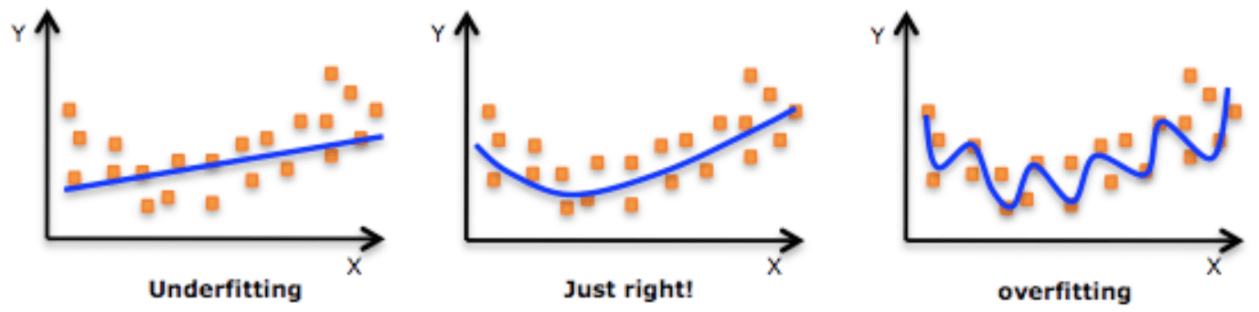
Figure 4: Representation of a model that is unverfitting, ok, and overfitting. Image source: https://www.datarobot.com/wp-content/uploads/2018/03/Screen-Shot-2018-03-22-at-11.22.15-AM-e1526498075543.png.
With the model we have just designed, the loss function of validation and training results is ok, what can be confirmed by a plot of their losses:
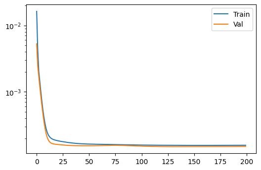
Figure 5: Train and validation losses for the model in question.
Testing the model
After all this work it is time to see how the model is performing on the test set:
lloss_test = []
preds = []
xss = []
yss = []
for x, y in test_loader:
  out = model( x.to(device))
  preds.append( out.detach().cpu().numpy() )
  xss.append( np.array( x ) )
  yss.append( np.array( y ) )
  loss = loss_func(out, torch.from_numpy( np.array(y[:, 0]) ).float().to(device))
lloss_test.append( loss.data.cpu().numpy() )

new_preds = np.concatenate( [preds[i] for i in range(len(preds))])
new_yss = np.concatenate( [yss[i] for i in range(len(yss))])
new_xss = np.concatenate( [xss[i] for i in range(len(xss))])

df = pd.DataFrame()

df["x_truth"] = new_xss[:, 0]*std + mean
df["y_truth"] = new_yss[:, 0]*(max - min) + min
df["y_pred"] = new_preds[:, 0]*(max - min) + min
And the analyses como with the loss for the test set:
loss_test = np.mean(lloss_test)
A histogram:
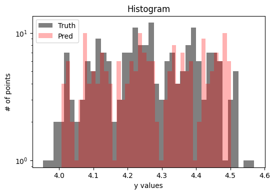
Figure 6: A histogram of the truch and test set predictions.
And a truth $\times$ predictions plot:
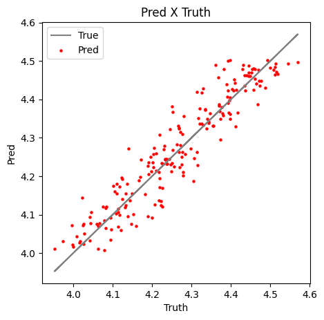
Figure 7: Predictions $\times$ Truth values for the test set.
As we can see by the plots above the model achieved good predictions, with a small dispersion over the pred $\times$ truth analysis. Anyhow, this is a really simple regression example, that I hope can help you to start having fun with PyTorch and machine learning.
Stay tunned for new posts!