How to simulate the Universe on a computer

Hello there! In this post, I will write a bit about cosmological simulations. Yes, it’s a promise-I’ve been meaning to do this since I created this blog, and it’s been a while since my last post.

Why do people try to simulate our Universe on computers?

First things first: we have always been passionate about understanding our Universe, and what better way to do so than by mimicking it using the tools we have: computational power and cosmology? But why rely on numerical simulations? Well, if you’ve read a bit about cosmology, you’ll know that understanding how matter behaves on small scales is quite challenging. The “simple theory” (linear cosmology) works remarkably well for describing large-scale structures (Gaussian fields), but it breaks down at smaller scales, where nonlinearities start to dominate.

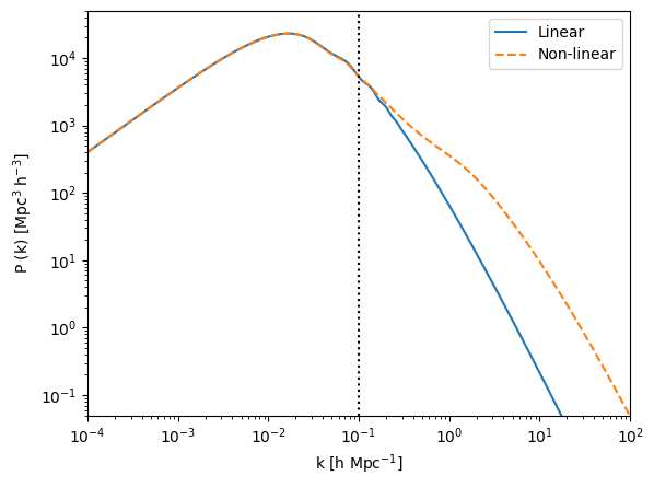
Figure 1: Linear and nonlinear power spectrum comparison. The spectra are presented for redshift zero. The impact of nonlinearities is evident starting from $k \gtrsim 0.1$ h/Mpc.

For example, in the case of the power spectrum - a summary statistic that describes how much matter (or power) exists at different scales ($k$) - we can use linear theory to model the distribution of matter up to $k \lesssim 0.1$ h/Mpc. Beyond this point, the power spectrum becomes nonlinear. See Figure 1.

To predict clustering on small scales, the main approach is through numerical simulations. These simulations employ high-resolution, multi-scale schemes and are routinely used on massively parallel computers to increase their size and complexity, aiming to better describe the Universe. Given the complexity of the Universe and its various components, these numerical solutions can be classified into two main categories: $N$-body (or DM-only) simulations and hydrodynamical (or DM plus baryons) simulations. $N$-body simulations involve solely DM, with gravity being the only force acting on the particles. On the other hand, hydrodynamical simulations incorporate both DM and baryonic matter (e.g., gas), allowing for the inclusion of phenomena such as feedback from supernova explosions and supermassive black holes (BH), magnetic effects, and more. Let’s discuss a bit more about both sets of simulations.

N-body simulations

$N$-body (or DM-only) simulations are numerical solutions of a very high number ($N$) of DM particles interacting gravitationally within a finite volume, and evolving over a long period of time (or a large range of redshifts). Essentially, they provide an alternative path to solutions of the collisionless Boltzmann equations coupled with Poisson’s equation. Examples of such simulations include the Millennium, Dark Sky, and Bolshoi simulations, which are widely used by the scientific community to study large-scale structures and the behavior of DM on large volumes. Another notable example is the Quijote project, which consists of a collection of $43,100$ full $N$-body simulations designed to provide an extensive data set of cosmological simulations for machine learning (ML) applications.

In this post I will present one of the techniques employed to solve the problem of simulating cosmological structures: the particle mesh (PM) algorithm. Other methods, such as particle-particle schemes or hybrid schemes, also exist, each with its own advantages and disadvantages.

The PM method is a relatively simple approach that I used myself when first delving into cosmology. I coded my own version of the method, largely following the principles outlined an amazing collection of notes from Dr. Andrey Kravtsov. PM codes utilize a mesh to represent density and potential fields, with the resolution of the simulation limited by the size of this mesh. Despite its simplicity, the PM method offers several advantages. It is fast, requiring fewer operations per particle per time step, compared to other methods. Additionally, PM simulations can handle very large numbers of particles efficiently.

Numerical N-body algorithms allow the study of nonlinear gravitational evolution of complex particle systems. These simulations model the time evolution of a given system by determining and tracking the trajectories of particles, taking into account their mutual gravitational interactions. Thus, a PM code solves both the Poisson equation $$\begin{equation} \nabla^2 \Phi = 4 \pi G \, \Omega_{m, 0} \, \rho_{crit} \, a^{- 1} \delta \, , \end{equation}$$ as well as the equations of motion of the particles, $$\begin{equation} \frac{d \mathbf{x}}{d a} = \frac{\mathbf{p}}{\dot{a} \, a^2} \end{equation}$$ $$\begin{equation} \frac{d \mathbf{p}}{d a} = - \frac{\mathbf{\nabla} \Phi}{\dot{a}} \, . \end{equation}$$

These equations are written in terms of comoving coordinates, i.e., $\mathbf{x} = \mathbf{r}/a$, where $\mathbf{r}$ represents the proper particle’s fluid position, and $\mathbf{p} = a \mathbf{v} = a^2 \dot{\mathbf{x}}$ denotes the particle momenta, where $$\begin{equation} \mathbf{v} = \mathbf{u} - H \mathbf{r} = a \dot{\mathbf{x}} \label{eq:pec_vel} \end{equation}$$ is the peculiar velocity, and $\mathbf{u}$ is the proper velocity (including the Hubble flow).

It is convenient to define code variables, i.e., dimensionless variables, that we will denote with tildes according to: $$\begin{equation} \tilde{\mathbf{x}} \equiv \frac{\mathbf{x}}{r_0} = \frac{\mathbf{r}}{a r_0} , \end{equation}$$
$$\begin{equation} \tilde{\mathbf{p}} \equiv \frac{\mathbf{p}}{v_0} = \frac{a \mathbf{v}}{v_0} , \end{equation}$$
$$\begin{equation} \tilde{\Phi} \equiv \frac{\Phi}{\phi_0} , \end{equation}$$
$$\begin{equation} \tilde{\rho} \equiv a^3 \frac{\rho}{\rho_0} . \end{equation}$$
The quantities with subscript zero correspond to physical variables responsible for removing the units from the code variables and are defined as $$\begin{equation} r_0 \equiv \frac{L_{BOX}}{N_g} , \end{equation}$$
$$\begin{equation} t_0 \equiv \frac{r_0}{t_0} , \end{equation}$$
$$\begin{equation} \rho_0 \equiv \rho_{crit} \Omega_{m, 0} , \end{equation}$$
$$\begin{equation} \Phi_0 \equiv \frac{r_0^2}{t_0^2} = v_0^2 , \end{equation}$$
where $L_{BOX}$ is the box size, measured in Mpc$/h$, $N_g$ is the number of grid cells in each direction, and $N_g^T = N_g^3$ is the total number of grid cells. In dimensionless variables, we can re-write the equations as $$\begin{equation} \tilde{\nabla}^2 \tilde{\Phi} = \frac{3}{2} \frac{\Omega_{m, 0}}{a}, \end{equation}$$
$$\begin{equation} \frac{d \tilde{\mathbf{x}}}{d a} = f (a) \frac{ \tilde{ \mathbf{p} } }{a^2} , \end{equation}$$
$$\begin{equation} \frac{d \tilde{\mathbf{p}}}{d a} = - f (a) \tilde{\mathbf{\nabla}} , \end{equation}$$
where $\tilde{\delta} = \tilde{\rho} - 1$ and $f (a) \equiv H_0/\dot{a}$.

The main idea of the PM code is to solve these equations in three main steps:

• Solve the Poisson Equation using the density field, estimated with current particle positions;
• Advance momenta $\tilde{\mathbf{p}}$, using the potential computed in the first step;
• Update particle positions $\tilde{\mathbf{x}}$, using the advanced momenta.

Implementation stage: solving the equations

The PM method exploits the fact that the Poisson equation for gravitational potential can be found in real space by convolving the density contrast with the Green’s function $$\begin{equation} \tilde{\phi} (\tilde{\mathbf{x}}) = \int d^3 \tilde{x}’ ~ G (\tilde{\mathbf{x}} - \tilde{\mathbf{x}}’) ~ \tilde{\delta} (\tilde{\mathbf{x}}’) . \end{equation}$$
The choice of the particular Green’s function $G$ is driven by the fact that we use periodic boundary conditions (PBC). In Fourier space, the convolution is then replaced by a simple multiplication: $$\begin{equation} \tilde{\phi} (\tilde{\mathbf{x}}) = G (\mathbf{k}) ~ \tilde{\delta} (\mathbf{k}) . \end{equation}$$ To obtain the density contrast $\tilde{\delta} (\mathbf{k})$ in Fourier space, first it is necessary to obtain $\tilde{\delta} (\tilde{\mathbf{x}})$ in real space, which arises from the density in real space $\tilde{\rho} (\tilde{\mathbf{x}})$.

The density field

In PM algorithms, particles are assumed to have a certain size, mass, shape, and internal density. This determines the interpolation scheme used to assign densities to grid cells. A common choice is the Cloud In Cell (CIC) method, where particles are represented as cubes (in $3$D) of uniform density and of one grid cell size.

The algorithm described above is relatively computationally cheap, accurate, and is commonly used in PM codes. In this method, the shape function of a particle in $1$ dimension is defined as $$\begin{equation} S (\tilde{x}) = \frac{1}{\Delta \tilde{x}} , |\tilde{x}| < \Delta \tilde{x}/2 \end{equation}$$ $$\begin{equation} S (\tilde{x}) = 0, otherwise, \end{equation}$$ for a cell size of $\Delta \tilde{x}$.
Then, the mass fraction of particle at $\tilde{x}_ p$, assigned to a cell at $\tilde{x}_ {i j k}$, is the shape function averaged over this cell: $$\begin{equation} W (\tilde{x}_ p - \tilde{x}_ {i j k}) = \int^{\tilde{x}_ {i j k} + \Delta \tilde{x}/2}_ {\tilde{x}_ {i j k} - \Delta \tilde{x}/2} d \tilde{x}’ ~ S (\tilde{x}_ p - \tilde{x}’) . \end{equation}$$ In $3$ dimensions this process generalizes to $$\begin{equation} W (\tilde{\mathbf{x}}_ p - \tilde{\mathbf{x}}_ {i j k}) = W (\tilde{x}_ p - \tilde{x}_ {i j k}) ~ W (\tilde{y}_ p - \tilde{y}_ {i j k}) ~ W (\tilde{z}_ p - \tilde{z}_ {i j k}) \, , \end{equation}$$ such that the density $\tilde{\rho}_ {i j k}$ in the corresponding cell is given by $$\begin{equation} \tilde{\rho}_ {i j k} = \sum^{N_p}_ {p = 1} \tilde{m}_ p W (\tilde{\mathbf{x}}_ p - \tilde{\mathbf{x}}_ {i j k}) , \end{equation}$$
where $N_ p^T = N_ p^3$ is the total number of particles, $N_ p$ is the number of particles “on each direction”, and $m_p$ is the particle mass. In practice, this is achieved by looping over particles and assigning their density to neighboring cells, rather than summing over all particles for each cell individually.

The density contrast field and its Fourier transform

With the grid densities $\tilde{\rho}_ {i, j, k} (\tilde{\mathbf{x}})$ on hand, the next step is to obtain the grid density contrasts $\tilde{\delta}_ {i, j, k} (\tilde{\mathbf{x}})$ and convert them to Fourier space. This transformation is typically accomplished using FFT algorithms, which efficiently compute the discrete Fourier Transform and its inverse. By applying the FFT to the grid density contrasts, we obtain the them in Fourier space, denoted as $\tilde{\delta}_ {i, j, k} (\tilde{\mathbf{k}})$.

The gravitational potential

Now we only need the Green function to obtain the gravitational field $\tilde{\Phi} (\mathbf{k})$. The Green function is given by $$\begin{equation} G (\mathbf{k}) = - \frac{3 \Omega_{m, 0}}{8 a} \left[ \sin^2 \left(\frac{k_x}{2}\right) + \sin^2\left(\frac{k_y}{2}\right) + \sin^2\left(\frac{k_z}{2}\right) \right]^{- 1} , \end{equation}$$ where $$\begin{equation} k_x = \frac{2 \pi l}{L_{BOX}} , \end{equation}$$ $$\begin{equation} k_y = \frac{2 \pi m}{L_{BOX}}, \end{equation}$$ $$\begin{equation} k_z = \frac{2 \pi n}{L_{BOX}}, \end{equation}$$ for the components $(l, m, n)$. These equations are in code units, hence $L_{BOX} = N_g$. Then, the gravitational potential is solved by transforming the result back to real space to obtain $\tilde{\Phi} (\tilde{\mathbf{x}})$ discretized at cell centers. Note that, when using these gravitational potentials, there is an artifact, a singularity at $l = m = n = 0$, which is avoided by setting $\tilde{\Phi}_{0 0 0} = 0$.

The acceleration

After obtaining the gravitational field in real space $\tilde{\Phi} (\tilde{\mathbf{x}})$, discretized at cell centers, it is time to obtain the acceleration at each grid point. This is simply given by $$\begin{equation} \tilde{\mathbf{a}} (\tilde{\mathbf{x_i}}) = - \tilde{\mathbf{\nabla}} \tilde{\Phi} (\tilde{\mathbf{x_i}}) \, . \end{equation}$$
This step precedes the updating of the particles’ positions and momenta, because it requires the accelerations at each particle’s position. Thus, to obtain the accelerations at the particle positions $\tilde{\mathbf{g}}^p$, we interpolate the acceleration at grid points $\tilde{\mathbf{a}} (\tilde{\mathbf{x_i}})$ onto the particle positions $\tilde{\mathbf{x}}_j^p$, using the CIC interpolation. During the density assignment, for a given particle, the acceleration at each point is interpolated from the cells to which the particle contributed to the density.

Updating particles positions and momenta

We arrive now at the final stage of the PM method: updating particle positions and momenta. This is achieved using leapfrog integration, which is a numerical method for integrating differential equations in a dynamical system. Leapfrog integration updates positions and velocities (or momenta) at interleaved time points (or scale factor points), staggered in such a way that they “leapfrog” over each other.

Thus, using the leapfrog integration, we have updated momenta and positions as $$\begin{equation} \tilde{\mathbf{p}}_ {n + 1/2} = \tilde{\mathbf{p}}_ {n - 1/2} + f (a_n) \tilde{\mathbf{g}}_ n \Delta a \end{equation}$$
$$\begin{equation} \tilde{\mathbf{x}}_ {n + 1} = \tilde{\mathbf{p}}_ {n} + a^{- 2}_ {n + 1/2} f (a_ {n + 1/2}) \tilde{\mathbf{p}}_ {n + 1/2} \Delta a , \end{equation}$$
where $n$ represents the “time” step, $f (a_n)$ is computed at $a_n$, $\Delta a$ is the step in the scalar factor, $$\begin{equation} a_n = a_i + n \Delta a \end{equation}$$
is the evolution in the scale factor according to the “time” steps, and $a_{n + 1/2} = a_n + \Delta a/2$. In the present case, we always update the momentum first, in a half time step before update the positions.

Therefore, the Particle Mesh (PM) method involves repeating a series of steps for each time step of the simulation. The main scheme of the PM method typically consists of the following three blocks, which are repeated iteratively:

• Find density on the mesh using the Cloud-In-Cell (CIC) technique. This step involves assigning the density of particles to grid cells using the CIC interpolation scheme.
• Solve the Poisson equation using two 3-dimensional Fast Fourier Transforms (FFTs). After obtaining the density distribution on the mesh, the Poisson equation is solved in Fourier space using FFTs to calculate the gravitational potential.
• Advance momenta and positions of the particles. Finally, the momenta and positions of the particles are updated using leapfrog integration based on the calculated gravitational potential.

These blocks are repeated for each time step of the simulation to evolve the system over time.

The simulations were conducted using the following cosmological parameters: $H_0 = 73.0$ km s$^{-1}$ Mpc$^{-1}$, $\Omega_{m} = 0.311051$, and $\Omega_{\Lambda} = 0.68887$. I ran four simulations, which explains the error bars seen in the final products, that I will present in a few minutes. I simulated a box of side $L_{BOX} = 128 ~ \text{Mpc}/h$, with $128^3$ particles and $256^3$ cells. The simulations started from $a = 0.02$ or $z = 49$, up to $a = 1.0$ or $z = 0$. The ICs were set using the Multi Scale Initial Conditions MUSIC(https://www-n.oca.eu/ohahn/MUSIC/) code. To define the initial spectra using MUSIC we utilized CAMB.

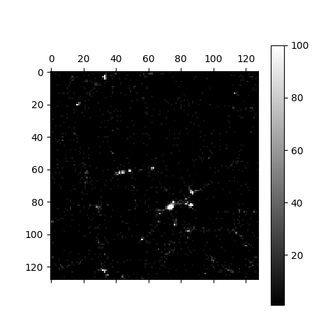
Figure 2: A snapshot of my $N$-body simulation. The animation can be seen in the youtube link

N-body power spectrum

The primary outcome obtained from the $N$-body simulation was the {\em power spectrum}, denoted as $P (k)$, at various stages and configurations of the simulation. Specifically, we computed the power spectrum based on FFTs performed on the density contrasts. We then calculated the quadratic modulus of these transformations and averaged the results over the $k$ values: $$\begin{equation} P (k) = \langle |\tilde{\delta} (k)|^2 \rangle = \frac{1}{N_k} \sum^{N_k}_ {i = 1} |\tilde{\delta} (k_i)|^2 , \end{equation}$$ where $i$ represents the bin index of $k$, i.e., $k_ i$ lies within the interval $[k, k + \Delta k]$, $k = \sqrt{k^2_ x + k^2_ y + k^2_ z}$, and $N_k$ represents the number of points where $k_i$ falls within the respective bin.

The power spectrum was computed for two distinct epochs: $a = 0.02$ and $a = 1.0$, to capture the evolution of the simulation. The results are illustrated in Figures 3 and 4, where a comparison is made with the linear and nonlinear spectra from CAMB. Error bars in the plots represent the standard deviation of the obtained spectra for four realizations of the simulation conducted under the fiducial Cosmology. Additionally, $\langle std\rangle$ denotes the average of these standard deviation values. The vertical lines denote the confidence interval of $k$ values, computed as $$\begin{equation} k_{min} = \frac{2 \pi}{L_{BOX}} \hspace{0.5cm}and\hspace{0.5cm} k_{max} = \frac{\pi N_p}{2 L_{BOX}} , \end{equation}$$ where $L_{BOX}$ is the size of the box of the simulation, $k_{min}$ is the minimum value of $k$ (also related to the simulation resolution), and $k_{max}$ is the maximum value of $k$, representing the Nyquist scale, which expresses the minimum separation between the particles.

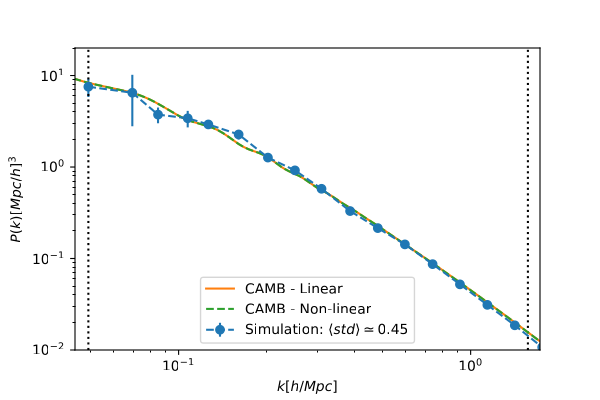
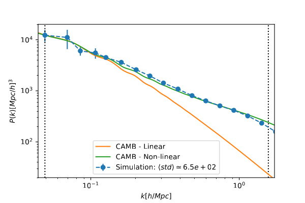
Figure 3: DM power spectrum from N-body simulation. The power spectrum is presented on the top, for $a = 0.02$ (or $z = 49$) and on the bottom for $a = 1.0$ (or $z = 0$). Both spectra were obtained for a box of side $L_ {BOX} = 128$ Mpc/h, with $N^T_p = 128^3$ particles, and $N^T_g = 2563$ cells. The vertical dotted lines indicate the maximum and minimum values for k. They are respectively: $k_ {min} \simeq 0.05$h/Mpc and $k_ {max} \simeq 1.57$h/Mpc. In both plots we compare the obtained power spectrum to the theoretical linear and nonlinear spectra from CAMB.

The overall trend of the power spectra aligns well with the model obtained from CAMB. Particularly, at $a = 0.02$, the spectrum matches exactly with the linear spectrum (and nonlinear as well, given the absence of structures at this stage). Conversely, at $a = 1.0$, the resulting spectrum closely resembles the nonlinear spectrum across all scales, indicating the emergence of structure and the breakdown of linear theory on small scales.

Approximated methods for DM simulations

$N$-body simulations are the state-of-art of gravitational dynamics for DM particles. However, their computational demands often limit their utility for extensive runs required for comparisons with real surveys, such as parameter estimation and covariance matrices. To address this challenge, numerous approximate methods have emerged to expedite results. Techniques like EZMocks, PINOCCHIO, ExSHalos, and others aim to generate DM halo catalogs using semi-analytical approximations or by emulating $N-$body simulations.

Hydrodynamical simulations

Hydrodynamical simulations play a pivotal role in comprehending galaxy formation and evolution in the Universe. Unlike DM-only simulations, hydrodynamical simulations incorporate ordinary matter, encompassing all components. As a result, they serve as the foundation of what we refer to as the halo-galaxy connection, directly bridging the information content between two key components: DM halos and galaxy properties. This integration is essential for deciphering a wide array of observed galaxy characteristics, including spatial clustering, mass distribution, stellar mass, size, color and star formation rate, among other properties.

Numerous recent initiatives are pushing the boundaries of hydrodynamical simulations, introducing new variations such as Astrid, SIMBA, IllustrisTNG, Magneticum, and SWIFT-EAGLE. A remarkable project is the CAMELS (Cosmology and Astrophysics with MachinE Learning Simulations) suite, comprising 12,903 cosmological simulations – 5,164 N-body and 7,712 state-of-the-art (magneto-)hydrodynamic simulations. Primarily designed to serve as a data set for ML analyses, CAMELS encompasses all the aforementioned simulations, focusing on small boxes of $25$ Mpc/h.

Indeed, while $N$-body simulations focus on the gravitational evolution of DM particles, hydrodynamical simulations encompass the evolution of all components, including the gravitational evolution of matter and the hydrodynamical evolution of gas. In some cases, these simulations also account for the interaction of gas with evolving radiation and magnetic fields. Initially, the baryon component, representing the visible Universe, consists mainly of gas, primarily hydrogen and helium. Some of this gas material ends up in stars during the process of structure formation. However, at the core of hydrodynamical simulations lie numerical solutions governing ideal, collisional, and non-conducting gases. Modeling the cosmic gas can be approached through three main branches: the Eulerian formulation, the Lagrangian formulation, or a hybrid of both. In the Lagrangian formulation, the following equations govern the fluid dynamics $$\begin{equation} \frac{D \rho}{D t} = - \rho \mathbf{\nabla} \cdot \mathbf{v} , \end{equation}$$ $$\begin{equation} \frac{D \mathbf{v}}{D t} = - \frac{1}{\rho} \mathbf{\nabla} P , \end{equation}$$ $$\begin{equation} \frac{D e}{D t} = \frac{1}{\rho} \mathbf{\nabla} \cdot p \mathbf{v} , \end{equation}$$ where $D/D t \equiv \partial/\partial t + \mathbf{v} \cdot \nabla$ denotes the Lagrangian derivative, $\rho$ is the density, $\mathbf{v}$ denotes de velocity vector, $P = (\gamma - 1) \rho u$ (with $\gamma$ being the heat capacity ratio and $u$ being the internal energy) denotes the thermodynamic pressure, and $e = u + \mathbf{v}^2/2$ is the total energy per unit mass.

This formulation assumes an observer that follows an individual fluid part, specified by its properties such as density $\rho$, as it moves through space and time. It can also be viewed as a mesh-free technique for approximating the continuum dynamics of fluids by samplings particles (an interpolation of points).

Due to limited numerical resolution of hydrodynamical simulations, which are among the most computationally expensive simulations in Cosmology and Astrophysics, certain physical processes must be included by hand. These processes are known as subgrid physical processes or sub-resolution models. They bridge the gap between the scales that can be treated numerically, typically above interstellar medium structure scales (around $3$ kpc), and those addressed by these subgrid routines, which extend below the scale of star clusters (around $0.3$ kpc). These subgrid models are a critical component of hydrodynamical simulations, introducing different parameters that must be tuned to ensure that their final products align with observational data.

It is not within the scope of the present thesis to delve into all the intricacies of subgrid physical processes. However, we can mention some of them, including:

• Gas cooling. This process dissipates the internal energy of gas through mechanisms such as ionization processes. It is often tabulated as a function of density, temperature, redshift, and composition for phenomena like photoionization. It is used by EAGLE and IllustrisTNG.
• Element abundance evolution. This process tracks the time release of individual elements from various nucleosynthetic channels. It is employed in simulations like SIMBA, Magneticum, EAGLE, and IllustrisTNG.
• Feedback processes. These processes involve the balance of inflows and outflows that regulate phenomena such as supernovae (SN) and active galactic nuclei (AGN) activity. They may be influenced by mechanisms like stellar winds and radiation pressure.
• Magnetic fields, cosmic rays, dust and others. These subgrid processes play crucial roles in shaping the evolution of galaxies and the intergalactic medium in hydrodynamical simulations.

Figure 4: A comparison of four hydrodynamic simulations (IllustrisTNG, SIMBA, Astrid and Magneticum) that have the same initial conditions but have been run with four different codes and subgrid models. Gas density and temperature are shown in blue and red colors, respectively. This showcase the different subgrid physics throught the different simulations. The link to video can be found here.

All these subgrid physical components require calibration, which is typically based on either physical arguments or observations – i.e., calibration aims at reproducing properties of galaxy populations. The most commonly used galaxy property for this calibration is the galaxy stellar mass, which is employed to calibrate feedback associated with stellar evolution. However, in simulations like EAGLE, galaxy size has also been used to reproduce galaxy scaling relations. Additionally, properties such as star formation rate and halo gas fractions are utilized in simulations like IllustrisTNG. It is important to note that the values chosen for these parameters may vary depending on the resolution of the simulation being considered. Consequently, this calibration serves as compelling evidence of the success of hydrodynamical simulations when compared to real observations.

Approximated methods to galaxies and halo-galaxy connection

As we have seen, hydrodynamic simulations represent the best of current simulation capabilities, as they provide a direct reproduction of observable properties of galaxies, which are (for the most part) the objects actually observed in the sky. Unlike DM halos, galaxies are baryonic entities, making hydrodynamic simulations invaluable for understanding their formation and evolution. However, these simulations are also the most computationally expensive, surpassing even $N$-body simulations in terms of computational resources required. Given their significance, there has been a concerted effort to develop approximate methods for predicting galaxy properties based on DM halo information. This subfield, often referred to as the halo-galaxy connection, aims at extracting galaxy-related information from DM halo simulations (or vice-versa).

The halo-galaxy connection refers to the relationship between the multivariate distribution of galaxy and halo properties derived from observations and simulations. Galaxies form and evolve within DM halos, and many of their properties are intrinsically related to the halo environment and clustering properties. For example, red galaxies tend to populate the centers of halos and are generally older, while blue galaxies are more often found in the outskirts of halos, and are typically younger. Modeling approaches to establish this link generally fall into two categories: physical and empirical models. Physical models include hydrodynamical simulations and Semi-Analytical Models (SAMs), which aim to capture the underlying physical processes governing galaxy formation within halos. On the other hand, empirical models such as Subhalo Abundance Matching (SHAM) and Halo Occupation Distribution (HOD) models are more data-driven and rely on statistical correlations between galaxy and halo properties observed in simulations or surveys.

SAMs approximate various physical processes using analytic prescriptions that can be tracked through the merger history of DM halos, and many codes are examples of this idea, such as Santa Cruz, GAEA, and L-Galaxies. SHAMs, on the other hand, establish a relationship between the mass of a galaxy and the abundance of the DM halos it typically inhabits. Finally, Decorated Halo Occupation Distribution models (decorated HODs) introduce additional halo properties besides mass, such as concentration, to determine the probability density distribution for the number of galaxies within their hosting halos.

Takeaway messages

$N$-body simulations model the gravitational interactions between a large number of particles, typically used to study the evolution of structures in the Universe, such as galaxy formation. These simulations track the motion of individual particles under the influence of gravity, providing insights into how large and small-scale structures evolve over time.

Hydrodynamic simulations, on the other hand, incorporate both gravity and the physics of fluids (gas dynamics), allowing for a more comprehensive modeling of astrophysical phenomena. These simulations are crucial for understanding the behavior of gas in galaxies, star formation, and other processes where matter is not just moving under gravity, but also undergoing physical interactions like pressure, temperature, and radiation.

Together, $N$-body and hydrodynamic simulations provide powerful tools for understanding the complex, dynamic Universe!